Chapter 5 Reliability

Too much consistency is as bad for the mind as it is for the body. Consistency is contrary to nature, contrary to life. The only completely consistent people are the dead.
— Aldous Huxley

Consistency is the hallmark of the unimaginative.
— Oscar Wilde

From the perspective of the creative thinker or innovator, consistency can be viewed as problematic. Consistent thinking leads to more of the same, as it limits diversity and change. On the other hand, inconsistent thinking or thinking outside the box produces new methods and ideas, inventions and breakthroughs, leading to innovation and growth.

Standardized tests are designed to be consistent, and, by their very nature, they tend to be poor measures of creative thinking. In fact, the construct of creativity is one of the more elusive in educational and psychological testing. Although published tests of creative thinking and problem solving exist, administration procedures are complex and consistency in the resulting scores can be, unsurprisingly, very low. Creativity seems to involve an inconsistency in thinking and behavior that is challenging to measure reliably.

From the perspective of the test maker or test taker, which happens to be the perspective we take in this book, consistency is critical to valid measurement. An inconsistent or unreliable test produces unreliable results that only inconsistently support the intended inferences of the test. Nearly a century of research provides us with a framework for examining and understanding the reliability of test scores, and, most importantly, how reliability can be estimated and improved.

This chapter introduces reliability within the framework of the classical test theory (CTT) model, which is then extended to generalizability (G) theory. In Chapter 7, we’ll learn about reliability within the item response theory model. These theories all involve measurement models, sometimes referred to as latent variable models, which are used to describe the construct or constructs assumed to underlie responses to test items.

This chapter starts with a general definition of reliability in terms of consistency of measurement. The CTT model and assumptions are then presented in connection with statistical inference and measurement models, which were introduced in Chapter 1. Reliability and unreliability, that is, the standard error of measurement, are discussed as products of CTT, and the four main study designs and corresponding methods for estimating reliability are reviewed. Finally, reliability is discussed for situations where scores come from raters. This is called interrater reliability, and it is best conceptualized using G theory.

Learning objectives

CTT reliability

1. Define reliability, including potential sources of reliability and unreliability in measurement, using examples.
2. Describe the simplifying assumptions of the classical test theory (CTT) model and how they are used to obtain true scores and reliability.
3. Identify the components of the CTT model (\(X\), \(T\), and \(E\)) and describe how they relate to one another, using examples.
4. Describe the difference between systematic and random error, including examples of each.
5. Explain the relationship between the reliability coefficient and standard error of measurement, and identify how the two are distinguished in practice.
6. Calculate the standard error of measurement and describe it conceptually.
7. Compare and contrast the three main ways of assessing reliability, test-retest, parallel-forms, and internal consistency, using examples, and identify appropriate applications of each.
8. Compare and contrast the four reliability study designs, based on 1 to 2 test forms and 1 to 2 testing occasions, in terms of the sources of error that each design accounts for, and identify appropriate applications of each.
9. Use the Spearman-Brown formula to predict change in reliability.
10. Describe the formula for coefficient alpha, the assumptions it is based on, and what factors impact it as an estimate of reliability.
11. Estimate different forms of reliability using statistical software, and interpret the results.
12. Describe factors related to the test, the test administration, and the examinees, that affect reliability.

Interrater reliability

13. Describe the purpose of measuring interrater reliability, and how interrater reliability differs from traditional reliability.
14. Describe the difference between interrater agreement and interrater reliability, using examples.
15. Calculate and interpret indices of interrater agreement and reliability, including proportion agreement, Kappa, Pearson correlation, and g coefficients.
16. Identify appropriate uses of each interrater index, including the benefits and drawbacks of each.
17. Describe the three main considerations involved in using g coefficients.

In this chapter, we’ll conduct reliability analyses on PISA09 data using epmr, and plot results using ggplot2. We’ll also simulate some data and examine interrater reliability using epmr.

# R setup for this chapter
# Required packages are assumed to be installed,
# see chapter 1
library("epmr")
library("ggplot2")
# Functions we'll use in this chapter
# set.seed(), rnorm(), sample(), and runif() to simulate
# data
# rowSums() for getting totals by row
# rsim() and setrange() from epmr to simulate and modify
# scores
# rstudy(), coef_alpha(), and sem() from epmr to get
# reliability and SEM
# geom_point(), geom_abline(), and geom_errorbar() for
# plotting
# diag() for getting the diagonal elements from a matrix
# astudy() from epmr to get interrater agreement
# gstudy() from epmr to run a generalizability study

5.1 Consistency of measurement

In educational and psychological testing, reliability refers to the precision of the measurement process, or the consistency of scores produced by a test. Reliability is a prerequisite for validity. That is, for scores to be valid indicators of the intended inferences or uses of a test, they must first be reliable or precisely measured. However, precision or consistency in test scores does not necessarily indicate validity.

A simple analogy may help clarify the distinction between reliability and validity. If the testing process is represented by an archery contest, where the test taker, an archer, gets multiple attempts to hit the center of a target, each arrow could be considered a repeated measurement of the construct of archery ability. Imagine someone whose arrows all end up within a few millimeters of one another, tightly bunched together, but all stuck in the trunk of a tree standing behind the target itself. This represents consistent but inaccurate measurement. On the other hand, consider another archer whose arrows are scattered around the target, with one hitting close to the bulls-eye and the rest spread widely around it. This represents measurement that is inconsistent and inaccurate, though more accurate perhaps than with the first archer. Reliability and validity are both present only when the arrows are all close to the center of the target. In that case, we’re consistently measuring what we intend to measure.

A key assumption in this analogy is that our archers are actually skilled, and any errors in their shots are due to the measurement process itself. Instead, consistently hitting a nearby tree may be evidence of a reliable test given to someone who is simply missing the mark because they don’t know how to aim. In reality, if someone scores systematically off target or above or below their true underlying ability, we have a hard time attributing this to bias in the testing process versus a true difference in ability.

A key point here is that evidence supporting the reliability of a test can be based on results from the test itself. However, evidence supporting the validity of the test must come, in part, from external sources. The only ways to determine that consistently hitting a tree represents low ability are to a) confirm that our test is unbiased and b) conduct a separate test. These are validity issues, which will be covered in Chapter 9.

Consider the reliability of other familiar physical measurements. One common example is measuring weight. How can measurements from a basic floor scale be both unreliable and invalid? Think about the potential sources of unreliability and invalidity. For example, consider measuring the weight of a young child every day before school. What is the variable we’re actually measuring? How might this variable change from day to day? And how might these changes be reflected in our daily measurements? If our measurements change from day to day, how much of this change can be attributed to actual changes in weight versus extraneous factors such as the weather or glitches in the scale itself?

In both of these examples, there are multiple interrelated sources of potential inconsistency in the measurement process. These sources of score change can be grouped into three categories. First, the construct itself may actually change from one measurement to the next. For example, this occurs when practice effects or growth lead to improvements in performance over time. Archers may shoot more accurately as they calibrate their bow or readjust for wind speed with each arrow. In achievement testing, students may learn or at least be refreshed in the content of a test as they take it.

Second, the testing process itself could differ across measurement occasions. Perhaps there is a strong cross-breeze one day but not the next. Or maybe the people officiating the competition allow for different amounts of time for warm-up. Or maybe the audience is rowdy or disagreeable at some points and supportive at others. These factors are tied to the testing process itself, and they may all lead to changes in scores.

Finally, our test may simply be limited in scope. Despite our best efforts, it may be that arrows differ from one another to some degree in balance or construction. Or it may be that archers’ fingers occasionally slip for no fault of their own. By using a limited number of shots, scores may change or differ from one another simply because of the limited nature of the test. Extending the analogy to other sports, football and basketball each involve many opportunities to score points that could be used to represent the ability of a player or team. On the other hand, because of the scarcity of goals in soccer, a single match may not accurately represent ability, especially when the referees have been bribed!

5.2 Classical test theory

5.2.1 The model

Now that we have a definition of reliability, with examples of the inconsistencies that can impact test scores, we can establish a framework for estimating reliability based on the changes or variability that occur in a set of test scores. Recall from Chapter 1 that statistics allow us to make an inference from a) the changes we observe in our test scores to b) what we assume is the underlying cause of these changes, the construct. Reliability is based on and estimated within a simple measurement model that decomposes an observed test score \(X\) into two parts, truth \(T\) and error \(E\):

\[\begin{equation} X = T + E. \tag{5.1} \end{equation}\]

Note that \(X\) in Equation (5.1) is a composite consisting of two component scores. The true score \(T\) is the construct we’re intending to measure. We assume that \(T\) is impacting our observation in \(X\). The error score \(E\) is everything randomly unrelated to the construct we’re intending to measure. Error also directly impacts our observation.

To understand the CTT model in Equation (5.1), we have to understand the following question: how would an individual’s observed score \(X\) vary across multiple repeated administrations of a test? If you took a test every day for the next 365 days, and somehow you forgot about all of the previous administrations of the test, would your observed score change from one testing to the next? And if so, why would it change?

CTT answers this question by making two key assumptions about the variability and covariability of \(T\) and \(E\). First, your true underlying ability \(T\) is assumed to be constant for an individual. If your true ability can be expressed as 20 out of 25 possible points, every time you take the test your true score will consistently be 20. It will not change, according to CTT. Second, error that influences an observed score at a given administration is assumed to be completely random, and thus unrelated to your true score and to any other error score for another administration.

So, at one administration of the test, some form of error may cause your score to decrease by two points. Maybe you weren’t feeling well that day. In this case, knowing that \(T = 20\), what is \(E\) in Equation (5.1), and what is \(X\)? At another administration, you might guess correctly on a few of the test questions, resulting in an increase of 3 based solely on error. What is \(E\) now? And what is \(X\)?

Solving for \(E\) in Equation (5.1) clarifies that random error is simply the difference between the true score and the observation, where a negative error always indicates that \(X\) is too low and a positive error always indicates that \(X\) is too high:

\[\begin{equation} E = X - T. \tag{5.2} \end{equation}\]

So, having a cold produces \(E = -2\) and \(X = 18\), compared to your true score of 20. And guessing correctly produces \(E = 3\) and \(X = 23\).

According to CTT, over infinite administrations of a test without practice effects, your true score will always be the same, and error scores will vary completely randomly, some being positive, others being negative, but being on average zero. Given these assumptions, what should your average observed score be across infinite administrations of the test? And what should be the standard deviation of your observed score over these infinite observed scores? In responding to these questions, you don’t have to identify specific values, but you should instead reference the means and standard deviations that you’d expect \(T\) and \(E\) to have. Remember that \(X\) is expressed entirely as a function of \(T\) and \(E\), so we can derive properties of the composite from its components.

# Simulate a constant true score, and randomly varying
# error scores from
# a normal population with mean 0 and SD 1
# set.seed() gives R a starting point for generating
# random numbers
# so we can get the same results on different computers
# You should check the mean and SD of E and X
# Creating a histogram of X might be interesting too
set.seed(160416)
myt <- 20
mye <- rnorm(1000, mean = 0, sd = 1)
myx <- myt + mye

Here is an explanation of the questions above. We know that your average observed score would be your true score. Error, because it varies randomly, would cancel itself out in the long run, and your mean \(X\) observed score would simply be \(T\). The standard deviation of these infinite observed scores \(X\) would then be entirely due to error. Since truth does not change, any change in observed scores must be error variability. This standard deviation is referred to as the standard error of measurement (SEM), discussed more below. Although it is theoretically impossible to obtain the actual SEM, since you can never take a test an infinite number of times, we can estimate SEM using data from a sample of test takers. And, as we’ll see below, reliability will be estimated as the opposite of measurement error.

Figure 5.1 presents the three pieces of the CTT model using PISA09 total reading scores for students from Belgium. We’re transitioning here from lots of \(X\) and \(E\) scores for an individual with a constant \(T\), to an \(X\), \(T\), and \(E\) score per individual within a sample. Total reading scores on the x-axis represent \(X\), and simulated \(T\) scores are on the y-axis. These total scores are calculated as \(T = X - E\). The solid line represents what we’d expect if there were no error, in which case \(X\) = \(T\). As a result, the horizontal scatter in the plot represents \(E\). Note that \(T\) are simulated to be continuous and to range from 0 to 11. \(X\) scores are discrete, but they’ve been “jittered” slightly left to right to reveal the densities of points in the plot.

# Calculate total reading scores, as in Chapter 2
ritems <- c("r414q02", "r414q11", "r414q06", "r414q09", 
  "r452q03", "r452q04", "r452q06", "r452q07", "r458q01",
  "r458q07", "r458q04")
rsitems <- paste0(ritems, "s")
xscores <- rowSums(PISA09[PISA09$cnt == "BEL", rsitems],
  na.rm = TRUE)
# Simulate error scores based on known SEM of 1.4, which
# we'll calculate later, then create true scores
# True scores are truncated to fall bewteen 0 and 11 using
# setrange()
escores <- rnorm(length(xscores), 0, 1.4)
tscores <- setrange(xscores - escores, y = xscores)
# Combine in a data frame and create a scatterplot
scores <- data.frame(x1 = xscores, t = tscores,
  e = escores)
ggplot(scores, aes(x1, t)) +
  geom_point(position = position_jitter(w = .3)) +
  geom_abline(col = "blue")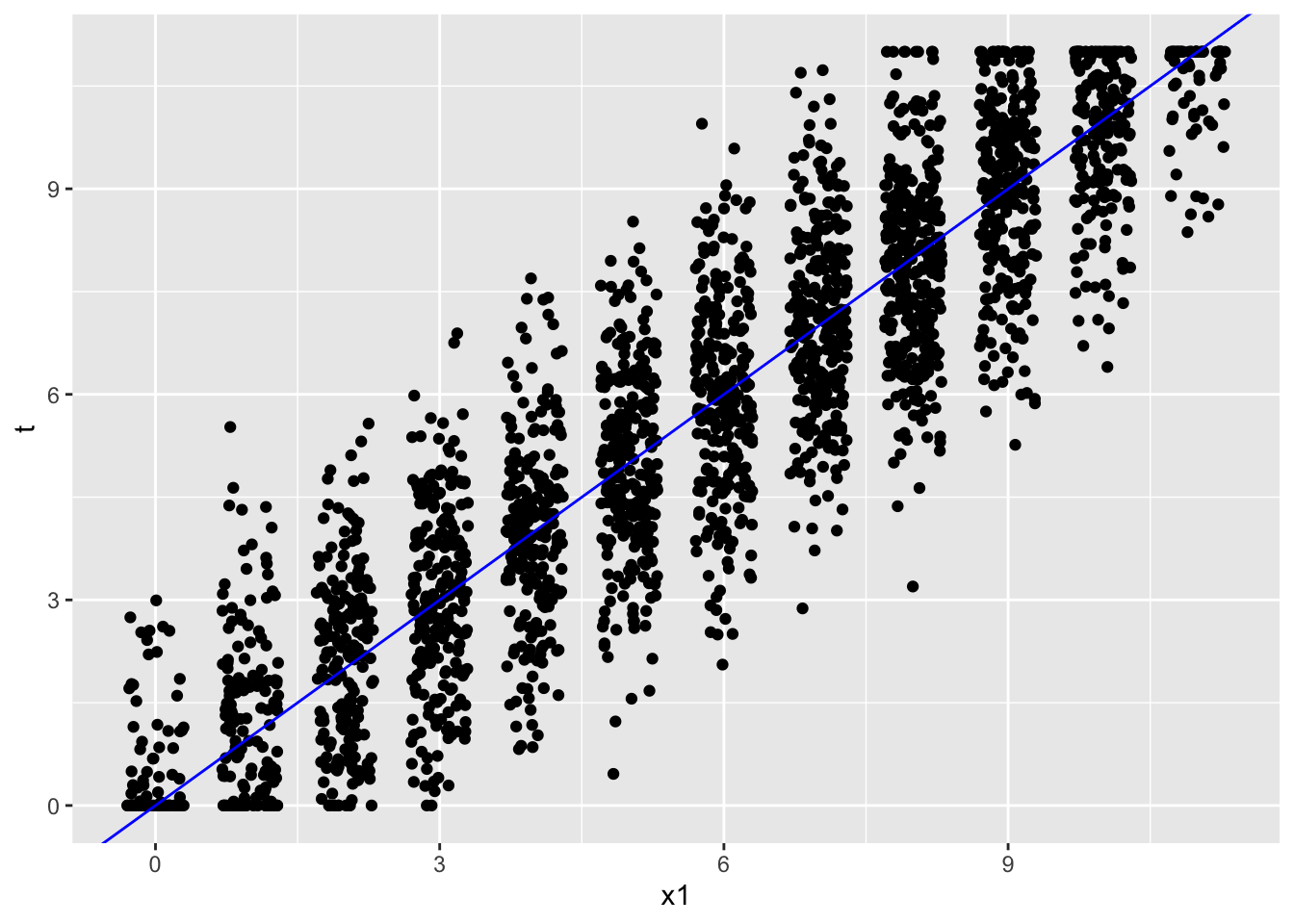

Figure 5.1: PISA total reading scores with simulated error and true scores based on CTT.

Consider individuals with a true score of \(T = 6\). The perfect test would measure true scores perfectly, and produce observed scores of \(X = T = 6\), on the solid line. In reality, lots of people scored at or around \(T = 6\), but their actual scores on \(X\) varied from about \(X = 3\) to \(X = 9\). Again, any horizontal distance from the blue line for a given true score represents \(E\).

5.2.2 Applications of the model

Let’s think about some specific examples now of the classical test theory model. Consider a construct that interests you, how this construct is operationalized, and the kind of measurement scale that results from it. Consider the possible score range, and try to articulate \(X\) and \(T\) in your own example.

Next, let’s think about \(E\). What might cause an individual’s observed score \(X\) to differ from their true score \(T\) in this situation? Think about the conditions in which the test would be administered. Think about the population of students, patients, individuals that you are working with. Would they tend to bring some form of error or unreliability into the measurement process?

Here’s a simple example involving preschoolers. As I mentioned in earlier chapters, some of my research involves measures of early literacy. In this research, we test children’s phonological awareness by presenting them with a target image, for example, an image of a star, and asking them to identify the image among three response options that rhymes with the target image. So, we’d present the images and say, “Which one rhymes with star?” Then, for example, children might point to the image of a car.

Measurement error is problematic in a test like this for a number of reasons. First of all, preschoolers are easily distracted. Even with standardized one-on-one test administration apart from the rest of the class, children can be distracted by a variety of seemingly innocuous features of the administration or environment, from the chair they’re sitting in, to the zipper on their jacket. In the absence of things in their environment, they’ll tell you about things from home, what they had for breakfast, what they did over the weekend, or, as a last resort, things from their imagination. Second of all, because of their short attention span, the test itself has to be brief and simple to administer. Shorter tests, as mentioned above in terms of archery and other sports, are less reliable tests; fewer items makes it more difficult to identify the reliable portion of the measurement process. In shorter tests, problems with individual items have a larger impact on the test as a whole.

Think about what would happen to \(E\) and the standard deviation of \(E\) if a test were very short, perhaps including only five test questions. What would happen to \(E\) and its standard deviation if we increased the number of questions to 200? What might happen to \(E\) and its standard deviation if we administered the test outside? These are the types of questions we will answer by considering the specific sources of measurement error and the impact we expect them to have, whether systematic or random, on our observed score.

5.2.3 Systematic and random error

A systematic error is one that influences a person’s score in the same way at every repeated administration. A random error is one that could be positive or negative for a person, or one that changes randomly by administration. In the preschooler literacy example, as students focus less on the test itself and more on their surroundings, their scores might involve more guessing, which introduces random error, assuming the guessing is truly random. Interestingly, we noticed in pilot studies of early literacy measures that some students tended to choose the first option when they didn’t know the correct response. This resulted in a systematic change in their scores based on how often the correct response happened to be first.

Distinguishing between systematic and random error can be difficult. Some features of a test or test administration can produce both types of error. A popular example of systematic versus random error is demonstrated by a faulty floor scale. Revisiting the example from above, suppose I measure my oldest son’s weight every day for two weeks as soon as he gets home from school. For context, my oldest is eleven years old at the time of writing this. Suppose also that his average weight across the two weeks was 60 pounds, but that this varied with a standard deviation of 5 pounds. Think about some reasons for having such a large standard deviation. What could cause my son’s weight, according to a floor scale, to differ from his true weight at a given measurement? What about his clothing? Or how many toys are in his pockets? Or how much food he ate for lunch?

What type of error does the standard deviation not capture? Systematic error doesn’t vary from one measurement to the next. If the scale itself is not calibrated correctly, for example, it may overestimate or underestimate weight consistently from one measure to the next. The important point to remember here is that only one type of error is captured by \(E\) in CTT: the random error. Any systematic error that occurs consistently across administrations will become part of \(T\), and will not reduce our estimate of reliability.

5.3 Reliability and unreliability

5.3.1 Reliability

Figure 5.2 contains a plot similar to the one in Figure 5.1 where we identified \(X\), \(T\), and \(E\). This time, we have scores on two reading test forms, with the first form is now called \(X_1\) and second form is \(X_2\), and we’re going to focus on the overall distances of the points from the line that goes diagonally across the plot. Once again, this line represents truth. A person with a true score of 11 on \(X_1\) will score 11 on \(X_2\), based on the assumptions of the CTT model.

Although the solid line represents what we’d expect to see for true scores, we don’t actually know anyone’s true score, even for those students who happen to get the same score on both test forms. The points in Figure 5.2 are all observed scores. The students who score the same on both test forms do indicate more consistent measurement. However, it could be that their true score still differs from observed. There’s no way to know. To calculate truth, we would have to administer the test an infinite number of times, and then take the average, or simply simulate it, as in Figure 5.1.

# Simulate scores for a new form of the reading test 
# called y
# rho is the made up reliability, which is set to 0.80
# x is the original reading total scores
# Form y is slightly easier than x with mean 6 and SD 3
xysim <- rsim(rho = .8, x = scores$x1, meany = 6, sdy = 3)
scores$x2 <- round(setrange(xysim$y, scores$x1))
ggplot(scores, aes(x1, x2)) +
  geom_point(position = position_jitter(w = .3, h = .3)) +
  geom_abline(col = "blue")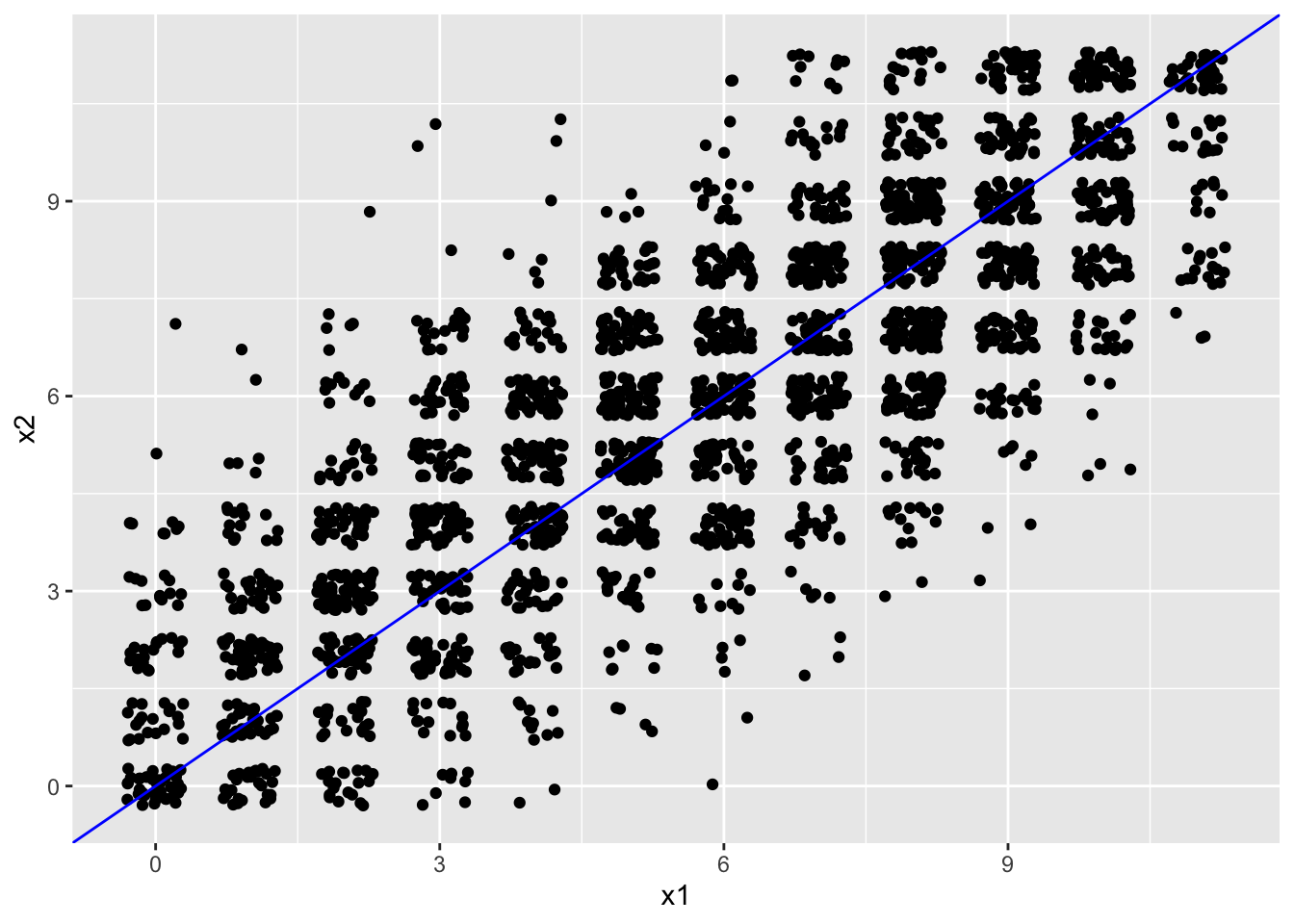

Figure 5.2: PISA total reading scores and scores on a simulated second form of the reading test.

The assumptions of CTT make it possible for us to estimate the reliability of scores using a sample of individuals. Figure 5.2 shows scores on two test forms, and the overall scatter of the scores from the solid line gives us an idea of the linear relationship between them. There appears to be a strong, positive, linear relationship. Thus, people tend to score similarly from one form to the next, with higher scores on one form corresponding to higher scores on the other. The correlation coefficient for this data set, cor(scores$x, scores$y) = 0.802, gives us an estimate of how similar scores are, on average from \(X_1\) to \(X_2\). Because the correlation is positive and strong for this plot, we would expect a person’s score to be pretty similar from one testing to the next.

Imagine if the scatter plot were instead nearly circular, with no clear linear trend from one test form to the next. The correlation in this case would be near zero. Would we expect someone to receive a similar score from one test to the next? On the other hand, imagine a scatter plot that falls perfectly on the line. If you score, for example, 10 on one form, you also score 10 on the other. The correlation in this case would be 1. Would we expect scores to remain consistent from one test to the next?

We’re now ready for a statistical definition of reliability. In CTT, reliability is defined as the proportion of variability in \(X\) that is due to variability in true scores \(T\):

\[\begin{equation} r = \frac{\sigma^2_T}{\sigma^2_X}. \tag{5.3} \end{equation}\]

Note that true scores are assumed to be constant in CTT for a given individual, but not across individuals. Thus, reliability is defined in terms of variability in scores for a population of test takers. Why do some individuals get higher scores than others? In part because they actually have higher abilities or true scores than others, but also, in part, because of measurement error. The reliability coefficient in Equation (5.3) tells us how much of our observed variability in \(X\) is due to true score differences.

5.3.2 Estimating reliability

Unfortunately, we can’t ever know the CTT true scores for test takers. So we have to estimate reliability indirectly. One indirect estimate made possible by CTT is the correlation between scores on two forms of the same test, as represented in Figure 5.2:

\[\begin{equation} r = \rho_{X_1 X_2} = \frac{\sigma_{X_1 X_2}}{\sigma_{X_1} \sigma_{X_2}}. \tag{5.4} \end{equation}\]

This correlation is estimated as the covariance, or the shared variance between the distributions on two forms, divided by a product of the standard deviations, or the total available variance within each distribution.

There are other methods for estimating reliability from a single form of a test. The only ones presented here are split-half reliability and coefficient alpha. Split-half is only presented because of its connection to what’s called the Spearman-Brown reliability formula. The split-half method predates coefficient alpha, and is computationally simpler. It takes scores on a single test form, and separates them into scores on two halves of the test, which are treated as separate test forms. The correlation between these two halves then represents an indirect estimate of reliability, based on Equation (5.3).

# Split half correlation, assuming we only had scores on 
# one test form
# With an odd number of reading items, one half has 5 
# items and the other has 6
xsplit1 <- rowSums(PISA09[PISA09$cnt == "BEL", 
  rsitems[1:5]])
xsplit2 <- rowSums(PISA09[PISA09$cnt == "BEL", 
  rsitems[6:11]])
cor(xsplit1, xsplit2, use = "complete")
## [1] 0.624843

The Spearman-Brown formula was originally used to correct for the reduction in reliability that occurred when correlating two test forms that were only half the length of the original test. In theory, reliability will increase as we add items to a test. Thus, Spearman-Brown is used to estimate, or predict, what the reliability would be if the half-length tests were made into full-length tests.

# sb_r() in the epmr package uses the Spearman-Brown 
# formula to estimate how reliability would change when 
# test length changes by a factor k
# If test length were doubled, k would be 2
sb_r(r = cor(xsplit1, xsplit2, use = "complete"), k = 2)
## [1] 0.7691119

The Spearman-Brown formula also has other practical uses. Today, it is most commonly used during the test development process to predict how reliability would change if a test form were reduced or increased in length. For example, if you are developing a test and you gather pilot data on 20 test items with a reliability estimate of 0.60, Spearman-Brown can be used to predict how this reliability would go up if you increased the test length to 30 or 40 items. You could also pilot test a large number of items, say 100, and predict how reliability would decrease if you wanted to use a shorter test.

The Spearman-Brown reliability, \(r_{new}\), is estimated as a function of what’s labeled here as the old reliability, \(r_{old}\), and the factor by which the length of \(X\) is predicted to change, \(k\):

\[\begin{equation} r_{new} = \frac{kr_{old}}{(k - 1)r_{old} + 1}. \tag{5.5} \end{equation}\]

Again, \(k\) is the factor by which the test length is increased or decreased. It is equal to the number of items in the new test divided by the number of items in the original test. Multiply \(k\) by the old reliability, and then divided the result by \((k - 1)\) times the old reliability, plus 1. For the example mentioned above, going from 20 to 30 items, we have \((30/20 \times 0.60)\) divided by \((30/20 - 1) \times 0.60 + 1 = 0.69\). Going to 40 items, we have a new reliability of 0.75. The epmr package contains sb_r(), a simple function for estimating the Spearman-Brown reliability.

Alpha is arguably the most popular form of reliability. Many people refer to it as “Chronbach’s alpha,” but Chronbach himself never intended to claim authorship for it and in later years he regretted the fact that it was attributed to him (see Cronbach and Shavelson 2004). The popularity of alpha is due to the fact that it can be calculated using scores from a single test form, rather than two separate administrations or split halves. Alpha is defined as

\[\begin{equation} r = \alpha = \left(\frac{J}{J - 1}\right)\left(\frac{\sigma^2_X - \sum\sigma^2_{X_j}}{\sigma^2_X}\right), \tag{5.6} \end{equation}\]

where \(J\) is the number of items on the test, \(\sigma^2_X\) is the variance of observed total scores on \(X\), and \(\sum\sigma^2_{X_j}\) is the sum of variances for each item \(j\) on \(X\). To see how it relates to the CTT definition of reliability in Equation (5.3), consider the top of the second fraction in Equation (5.6). The total test variance \(\sigma^2_X\) captures all the variability available in the total scores for the test. We’re subtracting from it the variances that are unique to the individual items themselves. What’s left over? Only the shared variability among the items in the test. We then divide this shared variability by the total available variability. Within the formula for alpha you should see the general formula for reliability, true variance over observed.

# epmr includes rstudy() which estimates alpha and a 
# related form of reliability called omega, along with 
# corresponding SEM
# You can also use coef_alpha() to obtain coefficient 
# alpha directly
rstudy(PISA09[, rsitems])
## 
## Reliability Study
## 
## Number of items: 11 
## 
## Number of cases: 44878 
## 
## Estimates:
##        coef  sem
## alpha 0.760 1.40
## omega 0.763 1.39

Keep in mind, alpha is an estimate of reliability, just like the correlation is. So, any equation requiring an estimate of reliability, like SEM below, can be computed using either a correlation coefficient or an alpha coefficient. Students often struggle with this point: correlation is one estimate of reliability, alpha is another. They’re both estimating the same thing, but in different ways based on different reliability study designs.

5.3.3 Unreliability

Now that we’ve defined reliability in terms of the proportion of observed variance that is true, we can define unreliability as the portion of observed variance that is error. This is simply 1 minus the reliability:

\[\begin{equation} 1 - r = \frac{\sigma^2_E}{\sigma^2_X}. \tag{5.7} \end{equation}\]

Typically, we’re more interested in how the unreliability of a test can be expressed in terms of the available observed variability. Thus, we multiply the unreliable proportion of variance by the standard deviation of \(X\) to obtain the SEM:

\[\begin{equation} SEM = \sigma_X\sqrt{1 - r}. \tag{5.8} \end{equation}\]

The SEM is the average variability in observed scores attributable to error. As any statistical standard error, it can be used to create a confidence interval (CI) around the statistic that it estimates, that is, \(T\). Since we don’t have \(T\), we instead create the confidence interval around \(X\) to index how confident we are that \(T\) falls within it for a given individual. For example, the verbal reasoning subtest of the GRE is reported to have a reliability of 0.93 and an SEM of 2.2, on a scale that ranges from 130 to 170. Thus, an observed verbal reasoning score of 155 has a 95% confidence interval of about \(\pm 4.4\) points. At \(X = 155\), we are 95% confident that the true score falls somewhere between 150.8 and 159.2. (Note that scores on the GRE are actually estimated using IRT.)

Confidence intervals for PISA09 can be estimated in the same way. First, we choose a measure of reliability, find the SD of observed scores, and obtain the corresponding SEM. Then, we can find the CI, which gives us the expected amount of uncertainty in our observed scores due to random measurement error. Here, we’re calculating SEM and the CI using alpha, but other reliability estimates would work as well. Figure 5.3 shows the 11 possible PISA09 reading scores in order, with error bars based on SEM for students in Belgium.

# Get alpha and SEM for students in Belgium
bela <- coef_alpha(PISA09[PISA09$cnt == "BEL", rsitems])$alpha
# The sem function from epmr sometimes overlaps with sem from 
# another R package so we're spelling it out here in long 
# form
belsem <- epmr::sem(r = bela, sd = sd(scores$x1,
  na.rm = T))
# Plot the 11 possible total scores against themselves
# Error bars are shown for 1 SEM, giving a 68% confidence
# interval and 2 SEM, giving the 95% confidence interval
# x is converted to factor to show discrete values on the 
# x-axis
beldat <- data.frame(x = 1:11, sem = belsem)
ggplot(beldat, aes(factor(x), x)) +
  geom_errorbar(aes(ymin = x - sem * 2,
    ymax = x + sem * 2), col = "violet") +
  geom_errorbar(aes(ymin = x - sem, ymax = x + sem),
    col = "yellow") +
  geom_point()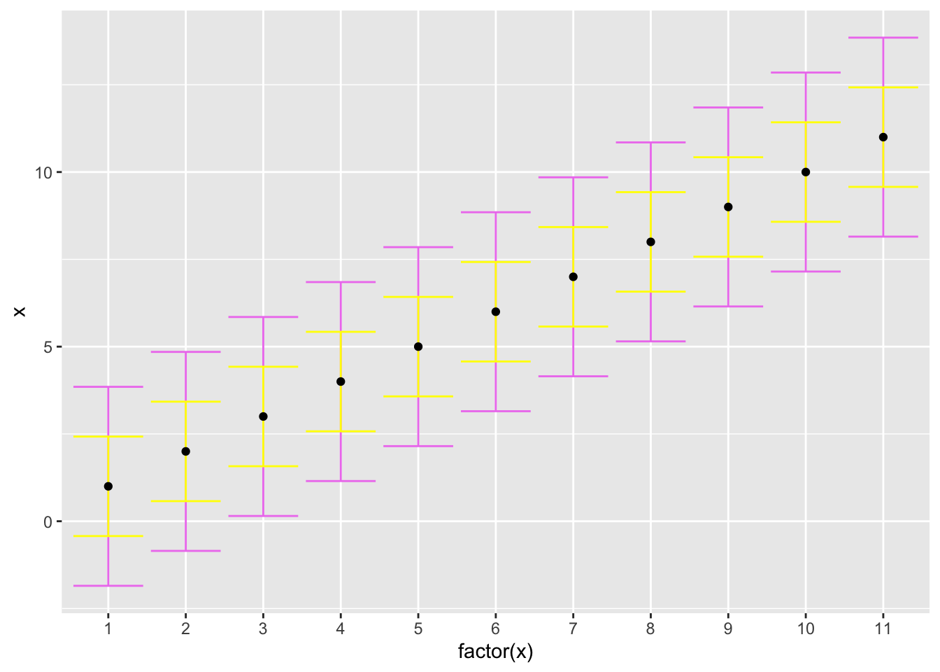

Figure 5.3: The PISA09 reading scale shown with 68 and 95 percent confidence intervals around each point.

Figure 5.3 helps us visualize the impact of unreliable measurement on score comparisons. For example, note that the top of the 95% confidence interval for \(X\) of 2 extends nearly to 5 points, and thus overlaps with the CI for adjacent scores 3 through 7. It isn’t until \(X\) of 8 that the CI no longer overlap. With a CI of belsem 1.425, we’re 95% confident that students with observed scores differing at least by belsem * 4 5.7 have different true scores. Students with observed scores closer than belsem * 4 may actually have the same true scores.

5.3.4 Interpreting reliability and unreliability

There are no agreed-upon standards for interpreting reliability coefficients. Reliability is bound by 0 on the lower end and 1 at the upper end, because, by definition, the amount of true variability can never be less or more than the total available variability in \(X\). Higher reliability is clearly better, but cutoffs for acceptable levels of reliability vary for different fields, situations, and types of tests. The stakes of a test are an important consideration when interpreting reliability coefficients. The higher the stakes, the higher we expect reliability to be. Otherwise, cutoffs depend on the particular application.

In general, reliabilities for educational and psychological tests can be interpreted using scales like the ones presented in Table 5.1. With medium-stakes tests, a reliability of 0.70 is sometimes considered minimally acceptable, 0.80 is decent, 0.90 is quite good, and anything above 0.90 is excellent. High stakes tests should have reliabilities at or above 0.90. Low stakes tests, which are often simpler and shorter than higher-stakes ones, often have reliabilities as low as 0.70. These are general guidelines, and interpretations can vary considerably by test. Remember that the cognitive measures in PISA would be considered low-stakes at the student level.

A few additional considerations are necessary when interpreting coefficient alpha. First, alpha assumes that all items measure the same single construct. Items are also assumed to be equally related to this construct, that is, they are assumed to be parallel measures of the construct. When the items are not parallel measures of the construct, alpha is considered a lower-bound estimate of reliability, that is, the true reliability for the test is expected to be higher than indicated by alpha. Finally, alpha is not a measure of dimensionality. It is frequently claimed that a strong coefficient alpha supports the unidimensionality of a measure. However, alpha does not index dimensionality. It is impacted by the extent to which all of the test items measure a single construct, but it does not necessarily go up or down as a test becomes more or less unidimensional.

Table 5.1: General Guidelines for Interpreting Reliability Coefficients

Reliability	High Stakes Interpretation	Low Stakes Interpretation
\(\geq 0.90\)	Excellent	Excellent
\(0.80 \leq r < 0.90\)	Good	Excellent
\(0.70 \leq r < 0.80\)	Acceptable	Good
\(0.60 \leq r < 0.70\)	Borderline	Acceptable
\(0.50 \leq r < 0.60\)	Low	Borderline
\(0.20 \leq r < 0.50\)	Unacceptable	Low
\(0.00 \leq r < 0.20\)	Unacceptable	Unacceptable

5.3.5 Reliability study designs

Now that we’ve established the more common estimates of reliability and unreliability, we can discuss the four main study designs that allow us to collect data for our estimates. These designs are referred to as internal consistency, equivalence, stability, and equivalence/stability designs. Each design produces a corresponding type of reliability that is expected to be impacted by different sources of measurement error.

The four standard study designs vary in the number of test forms and the number of testing occasions involved in the study. Until now, we’ve been talking about using two test forms on two separate administrations. This study design is found in the lower right corner of Table 5.2, and it provides us with an estimate of equivalence (for two different forms of a test) and stability (across two different administrations of the test). This study design has the potential to capture the most sources of measurement error, and it can thus produce the lowest estimate of reliability, because of the two factors involved. The more time that passes between administrations, and as two test forms differ more in their content and other features, the more error we would expect to be introduced. On the other hand, as our two test forms are administered closer in time, we move from the lower right corner to the upper right corner of Table 5.2, and our estimate of reliability captures less of the measurement error introduced by the passage of time. We’re left with an estimate of the equivalence between the two forms.

As our test forms become more and more equivalent, we eventually end up with the same test form, and we move to the first column in Table 5.2, where one of two types of reliability is estimated. First, if we administer the same test twice with time passing between administrations, we have an estimate of the stability of our measurement over time. Given that the same test is given twice, any measurement error will be due to the passage of time, rather than differences between the test forms. Second, if we administer one test only once, we no longer have an estimate of stability, and we also no longer have an estimate of reliability that is based on correlation. Instead, we have an estimate of what is referred to as the internal consistency of the measurement. This is based on the relationships among the test items themselves, which we treat as miniature alternate forms of the test. The resulting reliability estimate is impacted by error that comes from the items themselves being unstable estimates of the construct of interest.

Table 5.2: Four Main Reliability Study Designs

	1 Form	2 Forms
1 Occasion	Internal Consistency	Equivalence
2 Occasions	Stability	Equivalence & Stability

Internal consistency reliability is estimated using either coefficient alpha or split-half reliability. All the remaining cells in Table 5.2 involve estimates of reliability that are based on correlation coefficients.

Table 5.2 contains four commonly used reliability study designs. There are others, including designs based on more than two forms or more than two occasions, and designs involving scores from raters, discussed below.

5.4 Interrater reliability

It was like listening to three cats getting strangled in an alley.
— Simon Cowell, disparaging a singer on American Idol

Interrater reliability can be considered a specific instance of reliability where inconsistencies are not attributed to differences in test forms, test items, or administration occasions, but to the scoring process itself, where humans, or in some cases computers, contribute as raters. Measurement with raters often involves some form of performance assessment, for example, a stage performance within a singing competition. Judgment and scoring of such a performance by raters introduces additional error into the measurement process. Interrater reliability allows us to examine the negative impact of this error on our results.

Note that rater error is another factor or facet in the measurement process. Because it is another facet of measurement, raters can introduce error above and beyond error coming from sampling of items, differences in test forms, or the passage of time between administrations. This is made explicit within generalizability theory, discussed below. Some simpler methods for evaluating interrater reliability are introduced first.

5.4.1 Proportion agreement

The proportion of agreement is the simplest measure of interrater reliability. It is calculated as the total number of times a set of ratings agree, divided by the total number of units of observation that are rated. The strengths of proportion agreement are that it is simple to calculate and it can be used with any type of discrete measurement scale. The major drawbacks are that it doesn’t account for chance agreement between ratings, and it only utilizes the nominal information in a scale, that is, any ordering of values is ignored.

To see the effects of chance, let’s simulate scores from two judges where ratings are completely random, as if scores of 0 and 1 are given according to the flip of a coin. Suppose 0 is tails and 1 is heads. In this case, we would expect two raters to agree a certain proportion of the time by chance alone. The table() function creates a cross-tabulation of frequencies, also known as a crosstab. Frequencies for agreement are found in the diagonal cells, from upper left to lower right, and frequencies for disagreement are found everywhere else.

# Simulate random coin flips for two raters
# runif() generates random numbers from a uniform 
# distribution
flip1 <- round(runif(30))
flip2 <- round(runif(30))
table(flip1, flip2)
##      flip2
## flip1 0 1
##     0 5 8
##     1 9 8

Let’s find the proportion agreement for the simulated coin flip data. The question we’re answering is, how often did the coin flips have the same value, whether 0 or 1, for both raters across the 30 tosses? The crosstab shows this agreement in the first row and first column, with raters both flipping tails 5 times, and in the second row and second column, with raters both flipping heads 8 times. We can add these up to get 13, and divide by \(n = 30\) to get the percentage agreement.

Data for the next few examples were simulated to represent scores given by two raters with a certain correlation, that is, a certain reliability. Thus, agreement here isn’t simply by chance. In the population, scores from these raters correlated at 0.90. The score scale ranged from 0 to 6 points, with means set to 4 and 3 points for the raters 1 and 2, and SD of 1.5 for both. We’ll refer to these as essay scores, much like the essay scores on the analytical writing section of the GRE. Scores were also dichotomized around a hypothetical cut score of 3, resulting in either a “Fail” or “Pass.”

# Simulate essay scores from two raters with a population 
# correlation of 0.90, and slightly different mean scores,
# with score range 0 to 6
# Note the capital T is an abbreviation for TRUE
essays <- rsim(100, rho = .9, meanx = 4, meany = 3,
  sdx = 1.5, sdy = 1.5, to.data.frame = T)
colnames(essays) <- c("r1", "r2")
essays <- round(setrange(essays, to = c(0, 6)))
# Use a cut off of greater than or equal to 3 to determine
# pass versus fail scores
# ifelse() takes a vector of TRUEs and FALSEs as its first
# argument, and returns here "Pass" for TRUE and "Fail" 
# for FALSE
essays$f1 <- factor(ifelse(essays$r1 >= 3, "Pass", 
  "Fail"))
essays$f2 <- factor(ifelse(essays$r2 >= 3, "Pass", 
  "Fail"))
table(essays$f1, essays$f2)
##       
##        Fail Pass
##   Fail   19    0
##   Pass   27   54

The upper left cell in the table() output above shows that for 19 individuals, the two raters both gave “Fail.” In the lower right cell, the two raters both gave “Pass” 54 times. Together, these two totals represent the agreement in ratings, 73 . The other cells in the table contain disagreements, where one rater said “Pass” but the other said “Fail.” Disagreements happened a total of 27 times. Based on these totals, what is the proportion agreement in the pass/fail ratings?

Table 5.3 shows the full crosstab of raw scores from each rater, with scores from rater 1 (essays$r1) in rows and rater 2 (essays$r2) in columns. The bunching of scores around the diagonal from upper left to lower right shows the tendency for agreement in scores.

Table 5.3: Crosstab of Scores From Rater 1 in Rows and Rater 2 in Columns

	0	1	2	3	4	5	6
0	1	1	0	0	0	0	0
1	1	2	0	0	0	0	0
2	5	8	1	0	0	0	0
3	0	6	11	2	1	0	0
4	0	0	9	9	10	0	0
5	0	0	1	4	6	3	1
6	0	0	0	2	3	3	10

Proportion agreement for the full rating scale, as shown in Table 5.3, can be calculated by summing the agreement frequencies within the diagonal elements of the table, and dividing by the total number of people.

# Pull the diagonal elements out of the crosstab with 
# diag(), sum them, and divide by the number of people
sum(diag(table(essays$r1, essays$r2))) / nrow(essays)
## [1] 0.29

Finally, let’s consider the impact of chance agreement between one of the hypothetical human raters and a monkey who randomly applies ratings, regardless of the performance that is demonstrated, as with a coin toss.

# Randomly sample from the vector c("Pass", "Fail"), 
# nrow(essays) times, with replacement
# Without replacement, we'd only have 2 values to sample 
# from
monkey <- sample(c("Pass", "Fail"), nrow(essays),
  replace = TRUE)
table(essays$f1, monkey)
##       monkey
##        Fail Pass
##   Fail   10    9
##   Pass   38   43

The results show that the hypothetical rater agrees with the monkey 53 percent of the time. Because we know that the monkey’s ratings were completely random, we know that this proportion agreement is due entirely to chance.

5.4.2 Kappa agreement

Proportion agreement is useful, but because it does not account for chance agreement, it should not be used as the only measure of interrater consistency. Kappa agreement is simply an adjusted form of proportion agreement that takes chance agreement into account.

Equation (5.9) contains the formula for calculating kappa for two raters.

\[\begin{equation} \kappa = \frac{P_o - P_c}{1 - P_c} \tag{5.9} \end{equation}\]

To obtain kappa, we first calculate the proportion of agreement, \(P_o\), as we did with the proportion agreement. This is calculated as the total for agreement divided by the total number of people being rated. Next we calculate the chance agreement, \(P_c\), which involves multiplying the row and column proportions (row and column totals divided by the total total) from the crosstab and then summing the result, as shown in Equation (5.10).

\[\begin{equation} P_c = P_{first-row}P_{first-col} + P_{next-row}P_{next-col} + \dots + P_{last-row}P_{last-col} \tag{5.10} \end{equation}\]

You do not need to commit Equations (5.9) and (5.10) to memory. Instead, they’re included here to help you understand that kappa involves removing chance agreement from the observed agreement, and then dividing this observed non-chance agreement by the total possible non-chance agreement, that is, \(1 - P_c\).

The denominator for the kappa equation contains the maximum possible agreement beyond chance, and the numerator contains the actual observed agreement beyond chance. So, the maximum possible kappa is 1.0. In theory, we shouldn’t ever observe less agreement than than expected by chance, which means that kappa should never be negative. Technically it is possible to have kappa below 0. When kappa is below 0, it indicates that our observed agreement is below what we’d expect due to chance. Kappa should also be no larger than proportion agreement. In the example data, the proportion agreement decreased from 0.29 to 0.159 for kappa.

A weighted version of the kappa index is also available. Weighted kappa let us reduce the negative impact of partial disagreements relative to more extreme disagreements in scores, by taking into account the ordinal nature of a score scale. For example, in Table 5.3, notice that only the diagonal elements of the crosstab measure perfect agreement in scores, and all other elements measure disagreements, even the ones that are close together like 2 and 3. With weighted kappa, we can give less weight to these smaller disagreements and more weight to larger disagreements such as scores of 0 and 6 in the lower left and upper right of the table. This weighting ends up giving us a higher agreement estimate.

Here, we use the function astudy() from epmr to calculate proportion agreement, kappa, and weighted kappa indices. Weighted kappa gives us the highest estimate of agreement. Refer to the documentation for astudy() to see how the weights are calculated.

# Use the astudy() function from epmr to measure agreement
astudy(essays[, 1:2])
##     agree     kappa    wkappa 
## 0.2900000 0.1586681 0.4787490

5.4.3 Pearson correlation

The Pearson correlation coefficient, introduced above for CTT reliability, improves upon agreement indices by accounting for the ordinal nature of ratings without the need for explicit weighting. The correlation tells us how consistent raters are in their rank orderings of individuals. Rank orderings that are closer to being in agreement are automatically given more weight when determining the overall consistency of scores.

The main limitation of the correlation coefficient is that it ignores systematic differences in ratings when focusing on their rank orders. This limitation has to do with the fact that correlations are oblivious to linear transformations of score scales. We can modify the mean or standard deviation of one or both variables being correlated and get the same result. So, if two raters provide consistently different ratings, for example, if one rater is more forgiving overall, the correlation coefficient can still be high as long as the rank ordering of individuals does not change.

This limitation is evident in our simulated essay scores, where rater 2 gave lower scores on average than rater 1. If we subtract 1 point from every score for rater 2, the scores across raters will be more similar, as shown in Figure 5.4, but we still get the same interrater reliability.

# Certain changes in descriptive statistics, like adding 
# constants won't impact correlations
cor(essays$r1, essays$r2)
## [1] 0.8536149
dstudy(essays[, 1:2])
## 
## Descriptive Study
## 
##    mean median   sd   skew kurt min max   n na
## r1 3.86      4 1.49 -0.270 2.48   0   6 100  0
## r2 2.88      3 1.72  0.242 2.15   0   6 100  0
cor(essays$r1, essays$r2 + 1)
## [1] 0.8536149

A systematic difference in scores can be visualized by a consistent vertical or horizontal shift in the points within a scatter plot. Figure 5.4 shows that as scores are shifted higher for rater 2, they are more consistent with rater 1 in an absolute sense, despite the fact that the underlying linear relationship remains unchanged.

# Comparing scatter plots
ggplot(essays, aes(r1, r2)) +
  geom_point(position = position_jitter(w = .1, h = .1)) +
  geom_abline(col = "blue")
ggplot(essays, aes(r1, r2 + 1)) +
  geom_point(position = position_jitter(w = .1, h = .1)) +
  geom_abline(col = "blue")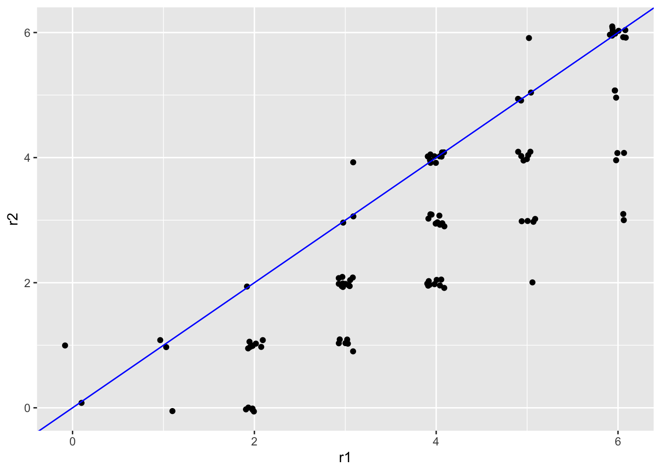

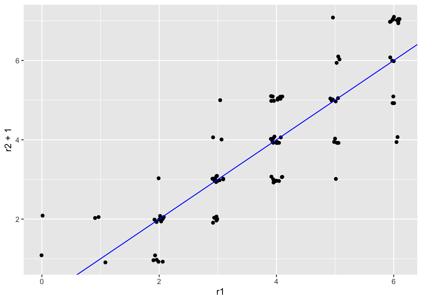
Figure 5.4: Scatter plots of simulated essay scores with a systematic difference around 0.5 points.

Is it a problem that the correlation ignores systematic score differences? Can you think of any real-life situations where it wouldn’t be cause for concern? A simple example is when awarding scholarships or giving other types of awards or recognition. In these cases consistent rank ordering is key and systematic differences are less important because the purpose of the ranking is to identify the top candidate. There is no absolute scale on which subjects are rated. Instead, they are rated in comparison to one another. As a result, a systematic difference in ratings would technically not matter.

5.5 Generalizability theory

Generalizability (G) theory addresses the limitations of other measures of reliability by providing a framework wherein systematic score differences can be accounted for, as well as the interactions that may take place in more complex reliability study designs. The G theory framework builds on the CTT model.

A brief introduction to G theory is given here, with a discussion of some key considerations in designing a G study and interpreting results. Resources for learning more include an introductory didactic paper by Brennan (1992), and textbooks by Shavelson and Webb (1991) and Brennan (2001).

5.5.1 The model

Recall from Equation (5.1) that in CTT the observed total score \(X\) is separated into a simple sum of the true score \(T\) and error \(E\). Given the assumptions of the model, a similar separation works with the total score variance:

\[\begin{equation} \sigma^2_X = \sigma^2_T + \sigma^2_E. \tag{5.11} \end{equation}\]

Because observed variance is simply the sum of true and error variances, we can rewrite the reliability coefficient in Equation (5.3) entirely in terms of true scores and error scores:

\[\begin{equation} r = \frac{\sigma^2_T}{\sigma^2_X} = \frac{\sigma^2_T}{\sigma^2_T + \sigma^2_E}. \tag{5.12} \end{equation}\]

Reliability in G theory, as in CTT, is considered to be the proportion of reliable score variance \(\sigma^2_T\) to reliable plus unreliable variance \(\sigma^2_T + \sigma^2_E\), that is, all score variance \(\sigma^2_X\).

In contrast to CTT, G theory breaks down the reliable variability into smaller pieces based on facets in the study design. Each facet is a feature of our data collection that we expect will lead to estimable variability in our total score \(X\). In CTT, there is only one facet, people. But G theory also allows us to account for reliable variability due to raters, among other things. As a result, Equations (5.1) and (5.11) are expanded or generalized in (5.13) and (5.14) so that the true score components are expressed as a combination of components for people \(P\) and raters \(R\).

\[\begin{equation} X = P + R + E \tag{5.13} \end{equation}\]

\[\begin{equation} \sigma^2_X = \sigma^2_P + \sigma^2_R + \sigma^2_E \tag{5.14} \end{equation}\]

5.5.2 Estimating generalizability

The breakdown of \(T\) into \(P\) and \(R\) in Equations (5.13) and (5.14) allows us to estimate reliability with what is referred to as a generalizability coefficient \(g\):

\[\begin{equation} g = \frac{\sigma^2_P}{\sigma^2_P + \sigma^2_R + \sigma^2_E}. \tag{5.15} \end{equation}\]

The G coefficient is an extension of CTT reliability in Equation (5.3), where the reliable variance of interest, formerly \(\sigma^2_T\), now comes from the people being measured, \(\sigma^2_P\). Reliable variance due to raters is then separated out in the denominator, and it is technically treated as a systematic component of our error scores. Note that, if there are no raters involved in creating observed scores, \(R\) disappears, \(T\) is captured entirely by \(P\), and Equation (5.15) becomes (5.3).

Generalizability coefficients can be estimated in a variety of ways. The epmr package includes functions for estimating a few different types of \(g\) using multilevel modeling via the lme4 package (Bates et al. 2015).

5.5.3 Applications of the model

If all of these equations are making your eyes cross, you should return to the question we asked earlier: why would a person score differently on a test from one administration to the next? The answer: because of differences in the person, because of differences in the rating process, and because of error. The goal of G theory is to compare the effects of these different sources on the variability in scores.

The definition of \(g\) in Equation (5.15) is a simple example of how we could estimate reliability in a person by rater study design. As it breaks down score variance into multiple reliable components, \(g\) can also be used in more complex designs, where we would expect some other facet of the data collection to lead to reliable variability in the scores. For example, if we administer two essays on two occasions, and at each occasion the same two raters provide a score for each subject, we have a fully crossed design with three facets: raters, tasks (i.e., essays), and occasions (e.g., Goodwin 2001). When developing or evaluating a test, we should consider the study design used to estimate reliability, and whether or not the appropriate facets are used.

In addition to choosing the facets in our reliability study, there are three other key considerations when estimating reliability with \(g\). The first consideration is whether we need to make absolute or relative score interpretations. Absolute score interpretations account for systematic differences in scores, whereas relative score interpretations do not. As mentioned above, the correlation coefficient considers only the relative consistency of scores, and it is not impacted negatively by systematic, that is, absolute, differences in scores. With \(g\), we may decide to adjust our estimate of reliability downward to account for these differences. The absolute reliability estimate from G theory is sometimes called the dependability coefficient \(d\).

The second consideration is the number of levels for each facet in our reliability study that will be present in operational administrations of the test. By default, reliability based on correlation is estimated for a single level of each facet. When we correlate scores on two test forms, the result is an estimate of the reliability of test itself, not some combination of two forms of the test. In the G theory framework, an extension of the Spearman-Brown formula can be used to predict increases or decreases in \(g\) based on increases or decreases in the number of levels for a facet. When Spearman-Brown was introduced in Equation (5.5), we considered changes in test length, where an increase in test length increased reliability. Now, we can also consider changes in the number of raters, or occasions, or any facet of our study. These predictions are referred to in the G theory literature as decision studies. The resulting \(g\) coefficients are labeled as average when more than one level is involved for a facet, and single otherwise.

The third consideration is the type of sampling used for each facet in our study, resulting in either random or fixed effects. Facets can be treated as either random samples from a theoretically infinite population, or as fixed, that is, not sampled from any larger population. Thus far, we have by default treated all facets as random effects. The people in our reliability study represent a broader population of people, as do raters. Fixed effects would be appropriate for facets with units or levels that will be used consistently and exclusively across operational administrations of a test. For example, in a study design with two essay questions, scored by two raters, we would treat the essay questions as fixed if we never intend to utilize other questions besides these two. Our questions are not samples from a population of potential essay questions. If instead our questions are simply two of many possible ones that could have been written or selected, it would be more appropriate to treat this facet in our study as a random effect. Fixing effects will increase reliability, as the error inherent in random sampling is eliminated from \(g\). Specifying random effects will then reduce reliability, as the additional error from random sampling is accounted for by \(g\).

The gstudy() function in the epmr package estimates variances and relative, absolute, single, and average \(g\) coefficients for reliability study designs with multiple facets, including fixed and random effects. Here, we’re simulating essay scores for a third rater in addition to the other two from the previous examples, and we’re examining the interrater reliability of this hypothetical testing example for all three raters at once. Without G theory, correlations or agreement indices would need to be computed for each pair of raters.

# Run a g study on simulated essay scores
essays$r3 <- rsim(100, rho = .9, x = essays$r2,
  meany = 3.5, sdy = 1.25)$y
essays$r3 <- round(setrange(essays$r3, to = c(0, 6)))
gstudy(essays[, c("r1", "r2", "r3")])
## 
## Generalizability Study
## 
## Call:
## gstudy.merMod(x = mer)
## 
## Model Formula:
## score ~ 1 + (1 | person) + (1 | rater)
## 
## Reliability:
##                       g    sem
## Relative Average 0.9368 0.3536
## Relative Single  0.8316 0.6125
## Absolute Average 0.8996 0.4546
## Absolute Single  0.7492 0.7874
## 
## Variance components:
##          variance  n1 n2
## person     1.8520 100  1
## rater      0.2449   3  3
## residual   0.3751  NA NA
## 
## Decision n:
## person  rater 
##    100      3

When given a data.frame object such as essays, gstudy() automatically assumes a design with one facet, comprising the columns of the data, where the units of observation are in the rows. Both rows and columns are treated as random effects. To estimate fixed effects for one or more facets, the formula interface for the function must instead be used. See the gstudy() documentation for details.

Our simulated ratings across three essays produce a relative average \(g\) of 0.937. This is interpreted as the consistency of scores that we’d expect in an operational administration of this test where an average essay score is taken over three raters. The raters providing scores are assumed to be sampled from a population of raters, and any systematic score differences over raters are ignored. The relative single \(g\) of 0.832 is interpreted as the consistency of scores that we’d expect if we decided to reduce the scoring process to just one rater, rather than all three. This single rater is still assumed to be sampled from a population, and systematic differences in scores are still ignored. The absolute average \(g\) 0.900 and absolute single \(g\) 0.749 are interpreted in the same way, but systematic score differences are taken into account, and the reliability estimates are thus lower than the relative ones.

5.6 Summary

This chapter provided an overview of reliability within the frameworks of CTT, for items and test forms, and G theory, for reliability study designs with multiple facets. After a general definition of reliability in terms of consistency in scores, the CTT model was introduced, and two commonly used indices of CTT reliability were discussed: correlation and coefficient alpha. Reliability was then presented as it relates to consistency of scores from raters. Interrater agreement indices were compared, along with the correlation coefficient, and an introduction to G theory was given.

5.6.1 Exercises

1. Explain the CTT model and its assumptions using the archery example presented at the beginning of the chapter.
2. Use the R object scores to find the average variability in x1 for a given value on t. How does this compare to the SEM?
3. Use PISA09 to calculate split-half reliabilities with different combinations of reading items in each half. Then, use these in the Spearman-Brown formula to estimate reliabilities for the full-length test. Why do the results differ?
4. Suppose you want to reduce the SEM for a final exam in a course you are teaching. Identify three sources of measurement error that could contribute to the SEM, and three that could not. Then, consider strategies for reducing error from these sources.
5. Estimate the internal consistency reliability for the attitude toward school scale. Remember to reverse code items as needed.
6. Dr. Phil is developing a measure of relationship quality to be used in counseling settings with couples. He intends to administer the measure to couples multiple times over a series of counseling sessions. Describe an appropriate study design for examining the reliability of this measure.
7. More and more TV shows lately seem to involve people performing some talent on stage and then being critiqued by a panel of judges, one of whom is British. Describe the ``true score’’ for a performer in this scenario, and identify sources of measurement error that could result from the judging process, including both systematic and random sources of error.
8. With proportion agreement, consider the following questions. When would we expect to see 0% or nearly 0% agreement, if ever? What would the counts in the table look like if there were 0% agreement? When would we expect to see 100% or nearly 100% agreement, if ever? What would the counts in the table look like if there were 100% agreement?
9. What is the maximum possible value for kappa? And what would we expect the minimum possible value to be?
10. Given the strengths and limitations of correlation as a measure of interrater reliability, with what type of score referencing is this measure of reliability most appropriate?
11. Compare the interrater agreement indices with interrater reliability based on Pearson correlation. What makes the correlation coefficient useful with interval data? What does it tell us, or what does it do, that an agreement index does not?
12. Describe testing examples where different combinations of the three G theory considerations are appropriate. For example, when would we want a G coefficient that captures reliability for an average across 2 raters, where raters are a random effect, ignoring systematic differences?

References

Bates, Douglas, Martin Mächler, Ben Bolker, and Steve Walker. 2015. “Fitting Linear Mixed-Effects Models Using lme4.” Journal of Statistical Software 67 (1): 1–48. https://doi.org/10.18637/jss.v067.i01.

Brennan, R. L. 1992. “Generalizability Theory.” Educational Measurement: Issues and Practice 11: 27–34.

Brennan, R. 2001. Generalizability Theory. New York, NY: Springer.

Cronbach, L J, and R. J. Shavelson. 2004. “My Current Thoughts on Coefficient Alpha and Successor Procedures.” Educational and Psychological Measurement 64: 391–418.

Goodwin, Laura D. 2001. “Interrater Agreement and Reliability.” Measurement in Physical Education and Exercise Science 5: 13–34.

Shavelson, R. J., and Norman L. Webb. 1991. Generalizability Theory: A Primer. SAGE Publications: Thousand Oaks, CA.