Chapter 7 Item Response Theory
One could make a case that item response theory is the most important statistical method about which most of us know little or nothing.
— David Kenny
Item response theory (IRT) is arguably one of the most influential developments in the field of educational and psychological measurement. IRT provides a foundation for statistical methods that are utilized in contexts such as test development, item analysis, equating, item banking, and computerized adaptive testing. Its applications also extend to the measurement of a variety of latent constructs in a variety of disciplines.
Given its role and influence in educational and psychological measurement, the topic of IRT has accumulated an extensive literature. Rather than cover every detail, this chapter gives a broad overview of IRT, with the intention of helping you understand key concepts and common applications. For comprehensive treatments of IRT, see de Ayala (2009) and Embretson and Reise (2000). For a comparison of CTT and IRT, see Hambleton and Jones (1993). Harvey and Hammer (1999) describe IRT specifically in the context of psychological testing.
This chapter begins with a comparison of IRT with classical test theory (CTT), including a discussion of strengths and weaknesses and some typical uses of each. Next, the traditional dichotomous IRT models are introduced with definitions of key terms and a comparison based on assumptions, benefits, limitations, and uses. Finally, details are provided on applications of IRT in item analysis, test development, item banking, and computerized adaptive testing.
Learning objectives
- Compare and contrast IRT and CTT in terms of their strengths and weaknesses.
- Identify the two main assumptions that are made when using a traditional IRT model, regarding dimensionality and functional form or the number of model parameters.
- Identify key terms in IRT, including probability of correct response, logistic curve, theta, and functions for item response, test response, standard error, and information.
- Define the three item parameters and one ability parameter in the traditional IRT models, and describe the role of each in modeling performance.
- Distinguish between the 1PL, 2PL, and 3PL IRT models in terms of assumptions made, benefits and limitations, and applications of each.
- Describe how IRT is utilized in item analysis, test development, item banking, and computer adaptive testing.
In this chapter, we’ll use epmr to run IRT analyses with PISA09 data, and we’ll use ggplot2 for plotting results.
# R setup for this chapter
library("epmr")
library("ggplot2")
# Functions we'll use in this chapter
# rirf() from epmr for getting an item response function
# scale_y_continuous() for plotting a continuous scale
# irtstudy() from epmr for running an IRT study
# rtef() from epmr for getting a test error function
# rtif() from epmr for getting a test information function
7.1 IRT versus CTT
Since its development in the 1950s and 1960s (Lord 1952; Rasch 1960), IRT has become the preferred statistical methodology for item analysis and test development. The success of IRT over its predecessor CTT comes primarily from the focus in IRT on the individual components that make up a test, that is, the items themselves. By modeling outcomes at the item level, rather than at the test level as in CTT, IRT is more complex but also more comprehensive in terms of the information it provides about test performance.
7.1.1 CTT review
As presented in Chapter 5, CTT gives us a model for the observed total score \(X\). This model decomposes \(X\) into two parts, truth \(T\) and error \(E\):
\[\begin{equation} X = T + E. \end{equation}\]
The true score \(T\) is the construct we’re intending to measure, and we assume it plays some systematic role in causing people to obtain observed scores on \(X\). The error \(E\) is everything randomly unrelated to the construct we’re intending to measure. Error also has a direct impact on \(X\). From Chapter 6, two item statistics that come from CTT are the mean performance on a given item, referred to as the \(p\)-value for dichotomous items, and the (corrected) item-total correlation for an item. Before moving on, you should be familiar with these two statistics, item difficulty and item discrimination, how they are related, and what they tell us about the items in a test.
It should be apparent that CTT is a relatively simple model of test performance. The simplicity of the model brings up its main limitation: the score scale is dependent on the items in the test and the people taking the test. The results of CTT are said to be sample dependent because 1) any \(X\), \(T\), or \(E\) that you obtain for a particular test taker only has meaning within the test she or he took, and 2) any item difficulty or discrimination statistics you estimate only have meaning within a particular sample of test takers. So, the person parameters are dependent on the test we use, and the item parameters are dependent on the test takers.
For example, suppose an instructor gives the same final exam to a new classroom of students each semester. At the first administration, the CITC discrimination for one item is 0.08. That’s low, and it suggests that there’s a problem with the item. However, in the second administration of the same exam to another group of students, the same item is found to have a CITC of 0.52. Which of these discriminations is correct? According to CTT, they’re both correct, for the sample with which they are calculated. In CTT there is technically no absolute item difficulty or discrimination that generalizes across samples or populations of examinees. The same goes for ability estimates. If two students take different final exams for the same course, each with different items but the same number of items, ability estimates will depend on the difficulty and quality of the respective exams. There is no absolute ability estimate that generalizes across samples of items. This is the main limitation of CTT: parameters that come from the model are sample and test dependent.
A second major limitation of CTT results from the fact that the model is specified using total scores. Because we rely on total scores in CTT, a given test only produces one estimate of reliability and, thus, one estimate of SEM, and these are assumed to be unchanging for all people taking the test. The measurement error we expect to see in scores would be the same regardless of level on the construct. This limitation is especially problematic when test items do not match the ability level of a particular group of people. For example, consider a comprehensive vocabulary test covering all of the words taught in a fourth grade classroom. The test is given to a group of students just starting fourth grade, and another group who just completed fourth grade and is starting fifth. Students who have had the opportunity to learn the test content should respond more reliably than students who have not. Yet, the test itself has a single reliability and SEM that would be used to estimate measurement error for any score. Thus, the second major limitation of CTT is that reliability and SEM are constant and do not depend on the construct.
7.1.2 Comparing with IRT
IRT addresses the limitations of CTT, the limitations of sample and test dependence and a single constant SEM. As in CTT, IRT also provides a model of test performance. However, the model is defined at the item level, meaning there is, essentially, a separate model equation for each item in the test. So, IRT involves multiple item score models, as opposed to a single total score model. When the assumptions of the model are met, IRT parameters are, in theory, sample and item independent. This means that a person should have the same ability estimate no matter which set of items she or he takes, assuming the items pertain to the same test. And in IRT, a given item should have the same difficulty and discrimination no matter who is taking the test.
IRT also takes into account the difficulty of the items that a person responds to when estimating the person’s ability or trait level. Although the construct estimate itself, in theory, does not depend on the items, the precision with which we estimate it does depend on the items taken. Estimates of the ability or trait are more precise when they’re based on items that are close to a person’s construct level. Precision decreases when there are mismatches between person construct and item difficulty. Thus, SEM in IRT can vary by the ability of the person and the characteristics of the items given.
The main limitation of IRT is that it is a complex model requiring much larger samples of people than would be needed to utilize CTT. Whereas in CTT the recommended minimum is 100 examinees for conducting an item analysis (see Chapter 6), in IRT, as many as 500 or 1000 examinees may be needed to obtain stable results, depending on the complexity of the chosen model.
# Prepping data for examples
# Create subset of data for Great Britain, then reduce to
# complete data
ritems <- c("r414q02", "r414q11", "r414q06", "r414q09",
  "r452q03", "r452q04", "r452q06", "r452q07", "r458q01",
  "r458q07", "r458q04")
rsitems <- paste0(ritems, "s")
PISA09$rtotal <- rowSums(PISA09[, rsitems])
pisagbr <- PISA09[PISA09$cnt == "GBR",
  c(rsitems, "rtotal")]
pisagbr <- pisagbr[complete.cases(pisagbr), ]
Another key difference between IRT and CTT has to do with the shape of the relationship that we estimate between item score and construct score. The CTT discrimination models a simple linear relationship between the two, whereas IRT models a curvilinear relationship between them. Recall from Chapter 6 that the discrimination for an item can be visualized within a scatter plot, with the construct on the \(x\)-axis and item scores on the \(y\)-axis. A strong positive item discrimination would be shown by points for incorrect scores bunching up at the bottom of the scale, and points for correct scores bunching up at the top. A line passing through these points would then have a positive slope. Because they’re based on correlations, ITC and CITC discriminations are always represented by a straight line with constant slope. See Figure 7.1 for an example based on PISA09 reading item r452q06s.
# Get p-values conditional on rtotal
# tapply() applies a function to the first argument over
# subsets of data defined by the second argument
pvalues <- data.frame(rtotal = 0:11,
  p = tapply(pisagbr$r452q06s, pisagbr$rtotal, mean))
# Plot CTT discrimination over scatter plot of scored item
# responses
ggplot(pisagbr, aes(rtotal, r414q06s)) +
  geom_point(position = position_jitter(w = 0.1,
    h = 0.1)) +
  geom_smooth(method = "lm", fill = NA) +
  geom_point(aes(rtotal, p), data = pvalues,
    col = "green", size = 3)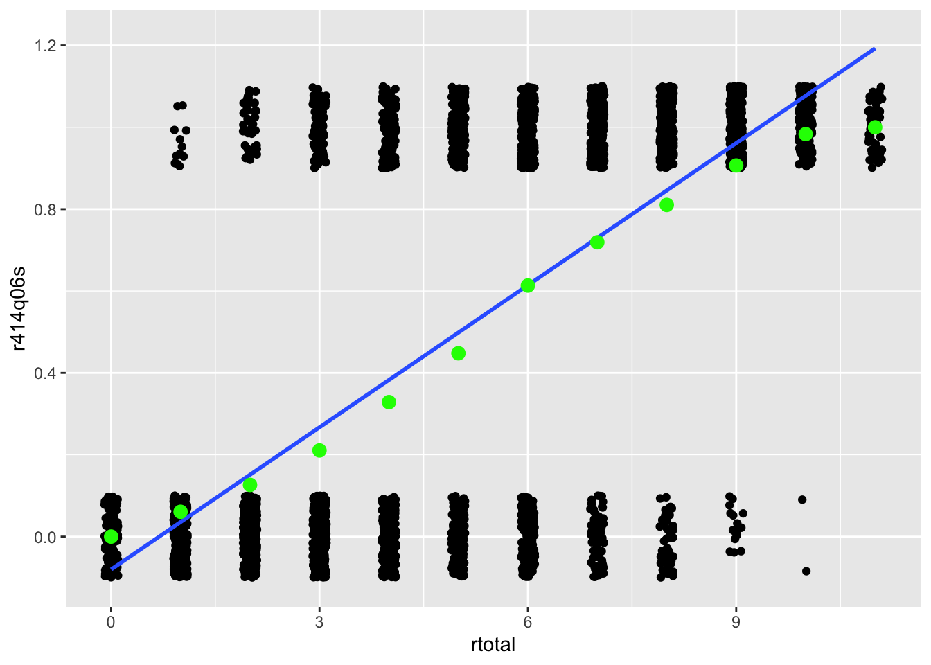
Figure 7.1: Scatter plots showing the relationship between total scores on the x-axis and scores from PISA item r452q06s on the y-axis. Lines represent the relationship between the construct and item scores for CTT (straight) and IRT (curved).
In IRT, the relationship between item and construct is similar to CTT, but the line follows what’s called a logistic curve. To demonstrate the usefulness of a logistic curve, we calculate a set of \(p\)-values for item r452q06s conditional on the construct. In Figure 7.1, the green points are \(p\)-values calculated within each group of people having the same total reading score. For example, the \(p\)-value on this item for students with a total score of 3 is about 0.20. As expected, people with lower totals have more incorrect than correct responses. As total scores increase, the number of people getting the item correct steadily increases. At a certain total score, around 5.5, we see roughly half the people get the item correct. Then, as we continue up the theta scale, more and more people get the item correct. IRT is used to capture the trend shown by the conditional \(p\)-values in Figure 7.1.
7.2 Traditional IRT models
7.2.1 Terminology
Understanding IRT requires that we master some new terms. First, in IRT the underlying construct is referred to as theta or \(\theta\). Theta refers to the same construct we discussed in CTT, reliability, and our earlier measurement models. The underlying construct is the unobserved variable that we assume causes the behavior we observe in item responses. Different test takers are at different levels on the construct, and this results in them having different response patterns. In IRT we model these response patterns as a function of the construct theta. The theta scale is another name for the ability or trait scale.
Second, the dependent variable in IRT differs from CTT. The dependent variable is found on the left of the model, as in a regression or other statistical model. The dependent variable in the CTT model is the total observed score \(X\). The IRT model instead has an item score as the dependent variable. The model then predicts the probability of a correct response for a given item, denoted \(\Pr(X = 1)\).
Finally, in CTT we focus only on the person construct \(T\) within the model itself. The dependent variable \(X\) is modeled as a function of \(T\), and whatever is left over via \(E\). In IRT, we include the construct, now \(\theta\), along with parameters for the item that characterize its difficulty, discrimination, and lower-asymptote.
In the discussion that follows, we will frequently use the term function. A function is simply an equation that produces an output for each input we supply to it. The CTT model could be considered a function, as each \(T\) has a single corresponding \(X\) that is influenced, in part, by \(E\). The IRT model also produces an output, but this output is now at the item level, and it is a probability of correct response for a given item. We can plug in \(\theta\), and get a prediction for the performance we’d expect on the item for that level on the construct. In IRT, this prediction of item performance depends on the item as well as the construct.
The IRT model for a given item has a special name in IRT. It’s called the item response function (IRF), because it can be used to predict an item response. Each item has its own IRF. We can add up all the IRF in a test to obtain a test response function (TRF) that predicts not item scores but total scores on the test.
Two other sets of functions, with corresponding equations, are also commonly used in IRT. The first is based on the contribution of an item, or set of items, to the reliability of measurement. In IRT, reliability is conceptualized using a statistical index called information. The item information function (IIF) tells us how reliability is expected to change for a given item when measuring across the theta scale. Remember that, whereas discrimination in CTT can be visualized with a straight line, the discrimination in IRT can be visualized with a curve. This curve is flatter at some points than others, indicating that an item is less discriminating at those points. In IRT, information tells us how the discriminating power of an item changes, thereby providing more and less reliable measurement, depending on theta. Multiple IIF can also be added together to get an overall test information function (TIF).
The last IRT function we’ll discuss here gives us the SEM for our test. This is called the test error function (TEF). As with all the other IRT functions, there is an equation that is used to estimate the function output, in this case, the standard error of measurement, for each point on the theta scale.
This overview of IRT terminology should help clarify the benefits of IRT over CTT. Recall that the main limitations of CTT are: 1) sample and test dependence, where our estimates of construct levels depend on the items in our test, and our estimates of item parameters depend on the construct levels for our sample of test takers; and 2) reliability and SEM that do not change depending on the construct. IRT addresses both of these limitations. The IRT model estimates the dependent variable of the model while accounting for both the construct and the properties of the item. As a result, estimates of ability or trait levels and item analysis statistics will be sample and test independent. This will be discussed further below. The IRT model also produces, via the IIF, TIF and TEF, measurement error estimates that vary by theta. Thus, the accuracy of a test depends on where the items are located on the construct.
Here’s a recap of the key terms we’ll be using throughout this chapter:
- Theta, \(\theta\), is our label for the construct measured for people.
- \(\Pr(X = 1)\) is the probability of correct response, the outcome in the IRT model. Remember that \(X\) is now an item score, as opposed to a total score in CTT.
- The IRF gives us a visual representation of \(\Pr(X = 1)\), showing predictions about how well people will do on an item based on theta.
- The logistic curve is the name for the shape we use to model performance via the IRF. It is a curve with certain properties, such as a slope that gradually increases and then decreases, and horizontal lower and upper asymptotes.
- The properties of the logistic curve are based on three item parameters, \(a\), \(b\), and \(c\), which are the item discrimination, difficulty, and lower-asymptote, also known as the pseudo-guessing parameter.
- Functions are simply equations that produce a single output value for each value on the theta scale. IRT functions include the IRF, TRF, IIF, TIF, and TEF.
- Information refers to the contribution of an item or test to the reliability of measurement.
7.2.2 The IRT models
We’ll now use the terminology above to compare three traditional IRT models. Equation (7.1) contains what is referred to as the three-parameter IRT model, because it includes all three available item parameters. The model is usually labeled 3PL, for 3 parameter logistic. As noted above, in IRT we model the probability of correct response on a given item (\(\Pr(X = 1)\)) as a function of person ability (\(\theta\)) and certain properties of the item itself, namely: \(a\), how well the item discriminates between low and high ability examinees; \(b\), how difficult the item is, or the construct level at which we’d expect people to have a probability \(\Pr = 0.50\) of getting the keyed item response; and \(c\), the lowest \(\Pr\) that we’d expect to see on the item by chance alone.
\[\begin{equation} \Pr(X = 1) = c + (1 - c)\frac{e^{a(\theta - b)}}{1 + e^{a(\theta - b)}} \tag{7.1} \end{equation}\]
The \(a\) and \(b\) parameters should be familiar. They are the IRT versions of the item analysis statistics from CTT, presented in Chapter 5. The \(a\) parameter corresponds to ITC, where larger \(a\) indicate larger, better discrimination. The \(b\) parameter corresponds to the opposite of the \(p\)-value, where a low \(b\) indicates an easy item, and a high \(b\) indicates a difficult item; higher \(b\) require higher \(\theta\) for a correct response. The \(c\) parameter should then be pretty intuitive if you think of its application to multiple-choice questions. When people low on the construct guess randomly on a multiple-choice item, the \(c\) parameter attempts to capture the chance of getting the item correct. In IRT, we acknowledge with the \(c\) parameter that the probability of correct response may never be zero. The smallest probability of correct response produced by Equation (7.1) will be \(c\).
To better understand the IRF in Equation (7.1), focus first on the difference we take between theta and item difficulty, in \((\theta - b)\). Suppose we’re using a cognitive test that measures some ability. If someone is high ability and taking a very easy item, with low \(b\), we’re going to get a large difference between theta and \(b\). This large difference filters through the rest of the equation to give us a higher prediction of how well the person will do on the item. This difference is multiplied by the discrimination parameter, so that, if the item is highly discriminating, the difference between ability and difficulty is magnified. If the discrimination is low, for example, 0.50, the difference between ability and difficulty is cut in half before we use it to determine probability of correct response. The fractional part and the exponential term represented by \(e\) serve to make the straight line of ITC into a nice curve with a lower and upper asymptote at \(c\) and 1. Everything on the right side of Equation (7.1) is used to estimate the left side, that is, how well a person with a given ability would do on a given item.
Figure 7.2 contains IRF for five items with different item parameters. Let’s examine the item with the IRF shown by the black line. This item would be considered the most difficult of this set, as it is located the furthest to the right. We only begin to predict that a person will get the item correct once we move past theta 0. The actual item difficulty, captured by the \(b\) parameter, is 3. This is found as the theta required to have a probability of 0.05 of getting the keyed response. This item also has the highest discrimination, as it is steeper than any other item. It is most useful for distinguishing between probabilities of correct response around theta 3, its \(b\) parameter; below and above this value, the item does not discriminate as well, as the IRF becomes more horizontal. Finally, this item appears to have a lower-asymptote of 0, suggesting test takers are likely not guessing on the item.
# Make up a, b, and c parameters for five items
# Get IRF using the rirf() function from epmr and plot
# rirf() will be demonstrated again later
ipar <- data.frame(a = c(2, 1, .5, 1, 1.5),
  b = c(3, 2, -.5, 0, -1),
  c = c(0, .2, .25, .1, .28),
  row.names = paste0("item", 1:5))
ggplot(rirf(ipar), aes(theta)) + scale_y_continuous("Pr(X)") +
  geom_line(aes(y = item1), col = 1) +
  geom_line(aes(y = item2), col = 2) +
  geom_line(aes(y = item3), col = 3) +
  geom_line(aes(y = item4), col = 4) +
  geom_line(aes(y = item5), col = 5)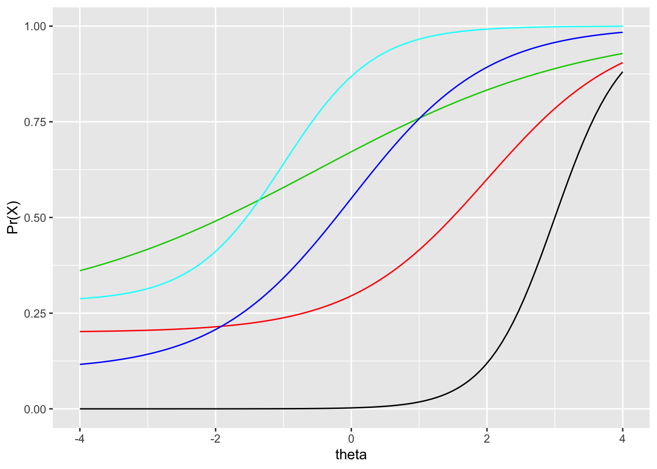
Figure 7.2: Comparison of five IRF having different item parameters.
Examine the remaining IRF in Figure 7.2. You should be able to compare the items in terms of easiness and difficulty, low and high discrimination, and low and high predicted probability of guessing correctly. Below are some specific questions and answers for comparing the items.
- Which item has the highest discrimination? Black, with the steepest slope.
- Which has the lowest discrimination? Green, with the shallowest slope.
- Which item is hardest, requiring the highest ability level, on average, to get it correct? Black, again, as it is furthest to the right.
- Which item is easiest? Cyan, followed by green, as they are furthest to the left.
- Which item are you most likely to guess correct? Green, cyan, and red appear to have the highest lower asymptotes.
Two other traditional, dichotomous IRT models are obtained as simplified versions of the three-parameter model in Equation (7.1). In the two-parameter IRT model or 2PL, we remove the \(c\) parameter and ignore the fact that guessing may impact our predictions regarding how well a person will do on an item. As a result,
\[\begin{equation} \Pr(X = 1) = \frac{e^{a(\theta - b)}}{1 + e^{a(\theta - b)}}. \tag{7.2} \end{equation}\]
In the 2PL, we assume that the impact of guessing is negligible. Applying the model to the items shown in Figure 7.2, we would see all the lower asymptotes pulled down to zero.
In the one-parameter model or 1PL, and the Rasch model (Rasch 1960), we remove the \(c\) and \(a\) parameters and ignore the impact of guessing and of items having differing discriminations. We assume that guessing is again negligible, and that discrimination is the same for all items. In the Rasch model, we also assume that discrimination is one, that is, \(a = 1\) for all items. As a result,
\[\begin{equation} \Pr(X = 1) = \frac{e^{(\theta - b)}}{1 + e^{(\theta - b)}}. \tag{7.3} \end{equation}\]
Zero guessing and constant discrimination may seem like unrealistic assumptions, but the Rasch model is commonly used operationally. The PISA studies, for example, utilize a form of Rasch modeling. The popularity of the model is due to its simplicity. It requires smaller sample sizes (100 to 200 people per item may suffice) than the 2PL and 3PL (requiring 500 or more people). The theta scale produced by the Rasch model can also have certain desirable properties, such as consistent score intervals (see de Ayala 2009).
7.2.3 Assumptions
The three traditional IRT models discussed above all involve two main assumptions, both of them having to do with the overall requirement that the model we chose is “correct” for a given situation. This correctness is defined based on 1) the dimensionality of the construct, that is, how many constructs are causing people to respond in a certain way to the items, and 2) the shape of the IRF, that is, which of the three item parameters are necessary for modeling item performance.
In Equations (7.1), (7.2), and (7.3) we have a single \(\theta\) parameter. Thus, in these IRT models we assume that a single person attribute or ability underlies the item responses. As mentioned above, this person parameter is similar to the true score parameter in CTT. The scale range and values for theta are arbitrary, so a \(z\)-score metric is typically used. The first IRT assumption then is that a single attribute underlies the item response process. The result is called a unidimensional IRT model.
The second assumption in IRT is that we’ve chosen the correct shape for our IRF. This implies that we have a choice regarding which item parameters to include, whether only \(b\) in the 1PL or Rasch model, \(b\) and \(a\) in the 2PL, or \(b\), \(a\), and \(c\) in the 3PL. So, in terms of shape, we assume that there is a nonlinear relationship between ability and probability of correct response, and this nonlinear relationship is captured completely by up to three item parameters.
Note that anytime we assume a given item parameter, for example, the \(c\) parameter, is unnecessary in a model, it is fixed to a certain value for all items. For example, in the Rasch and two-parameter IRT models, the \(c\) parameter is typically fixed to 0, which means we are assuming that guessing is not an issue. In the Rasch model we also assume that all items discriminate in the same way, and \(a\) is fixed to 1; then, the only item parameter we estimate is item difficulty.
7.3 Applications
7.3.1 In practice
As is true when comparing other statistical models, the choice of Rasch, 1PL, 2PL, or 3PL should be based on considerations of theory, model assumptions, and sample size.
Because of its simplicity and lower sample size requirements, the Rasch model is commonly used in small-scale achievement and aptitude testing, for example, with assessments developed and used at the district level, or instruments designed for use in research or lower-stakes decision-making. The IGDI measures discussed in Chapter 2 are developed using the Rasch model. The MAP tests, published by Northwest Evaluation Association, are also based on a Rasch model. Some consider the Rasch model most appropriate for theoretical reasons. In this case, it is argued that we should seek to develop tests that have items that discriminate equally well; items that differ in discrimination should be replaced with ones that do not. Others utilize the Rasch model as a simplified IRT model, where the sample size needed to accurately estimate different item discriminations and lower asymptotes cannot be obtained. Either way, when using the Rasch model, we should be confident in our assumption that differences between items in discrimination and lower asymptote are negligible.
The 2PL and 3PL models are often used in larger-scale testing situations, for example, on high-stakes tests such as the GRE and ACT. The large samples available with these tests support the additional estimation required by these models. And proponents of the two-parameter and three-parameter models often argue that it is unreasonable to assume zero lower asymptote, or equal discriminations across items.
In terms of the properties of the model itself, as mentioned above, IRT overcomes the CTT limitation of sample and item dependence. As a result, ability estimates from an IRT model should not depend on the sample of items used to estimate ability, and item parameter estimates should not depend on the sample of people used to estimate them. An explanation of how this is possible is beyond the scope of this book. Instead, it is important to remember that, in theory, when IRT is correctly applied, the resulting parameters are sample and item independent. As a result, they can be generalized across samples for a given population of people and test items.
IRT is useful first in item analysis, where we pilot test a set of items and then examine item difficulty and discrimination, as discussed with CTT in Chapter 6. The benefit of IRT over CTT is that we can accumulate difficulty and discrimination statistics for items over multiple samples of people, and they are, in theory, always expressed on the same scale. So, our item analysis results are sample independent. This is especially useful for tests that are maintained across more than one administration. Many admissions tests, for example, have been in use for decades. State tests, as another example, must also maintain comparable item statistics from year to year, since new groups of students take the tests each year.
Item banking refers to the process of storing items for use in future, potentially undeveloped, forms of a test. Because IRT allows us to estimate sample independent item parameters, we can estimate parameters for certain items using pilot data, that is, before the items are used operationally. This is what happens in a computer adaptive test. For example, the difficulty of a bank of items is known, typically from pilot administrations. When you sit down to take the test, an item of known average difficulty can then be administered. If you get the item correct, you are given a more difficult item. The process continues, with the difficulty of the items adapting based on your performance, until the computer is confident it has identified your ability level. In this way, computer adaptive testing relies heavily on IRT.
7.3.2 Examples
The epmr package contains functions for estimating and manipulating results from the Rasch model. Other R packages are available for estimating the 2PL and 3PL (e.g., Rizopoulos 2006). Commercial software packages are also available, and are often used when IRT is applied operationally.
Here, we estimate the Rasch model for PISA09 students in Great Britain. The data set was created at the beginning of the chapter. The irtstudy() function in epmr runs the Rasch model and prints some summary results, including model fit indices and variability estimates for random effect. Note that the model is being fit as a generalized linear model with random person and random item effects, using the lme4 package (Bates et al. 2015). The estimation process won’t be discussed here. For details, see Doran et al. (2007) and De Boeck et al. (2011).
# The irtstudy() function estimates theta and b parameters
# for a set of scored item responses
irtgbr <- irtstudy(pisagbr[, rsitems])
irtgbr
##
## Item Response Theory Study
##
## 3650 people, 11 items
##
## Model fit with lme4::glmer
##         AIC         BIC      logLik    deviance df.residual
##    46615.11    46632.31   -23305.55    38745.73    40148.00
##
## Random effects
##         Std.Dev      Var
## person 1.287442 1.657506
## item   1.011468 1.023067
The R object returned by irtstudy() contains a list of results. The first element in the list, irtgbr$data, contains the original data set with additional columns for the theta estimate and SEM for each person. The next element in the output list, irtgbr$ip, contains a matrix of item parameter estimates, with the first column fixed to 1 for \(a\), the second column containing estimates of \(b\), and the third column fixed to 0 for \(c\).
head(irtgbr$ip)
##          a           b c
## r414q02s 1 -0.02535278 0
## r414q11s 1  0.61180610 0
## r414q06s 1 -0.11701587 0
## r414q09s 1 -0.96943042 0
## r452q03s 1  2.80576876 0
## r452q04s 1 -0.48851334 0
Figure 7.3 shows the IRF for a subset of the PISA09 reading items based on data from Great Britain. These items pertain to the prompt “The play’s the thing” in Appendix C.2. Item parameters are taken from irtgbr$ip and supplied to the rirf() function from epmr. This function is simply Equation (7.1) translated into R code. Thus, when provided with item parameters and a vector of thetas, rirf() returns the corresponding \(\Pr(X = 1)\).
# Get IRF for the set of GBR reading item parameters and a
# vector of thetas
# Note the default thetas of seq(-4, 4, length = 100)
# could also be used
irfgbr <- rirf(irtgbr$ip, seq(-6, 6, length = 100))
# Plot IRF for items r452q03s, r452q04s, r452q06s, and
# r452q07s
ggplot(irfgbr, aes(theta)) + scale_y_continuous("Pr(X)") +
  geom_line(aes(y = irfgbr$r452q03s, col = "r452q03")) +
  geom_line(aes(y = irfgbr$r452q04s, col = "r452q04")) +
  geom_line(aes(y = irfgbr$r452q06s, col = "r452q06")) +
  geom_line(aes(y = irfgbr$r452q07s, col = "r452q07")) +
  scale_colour_discrete(name = "item")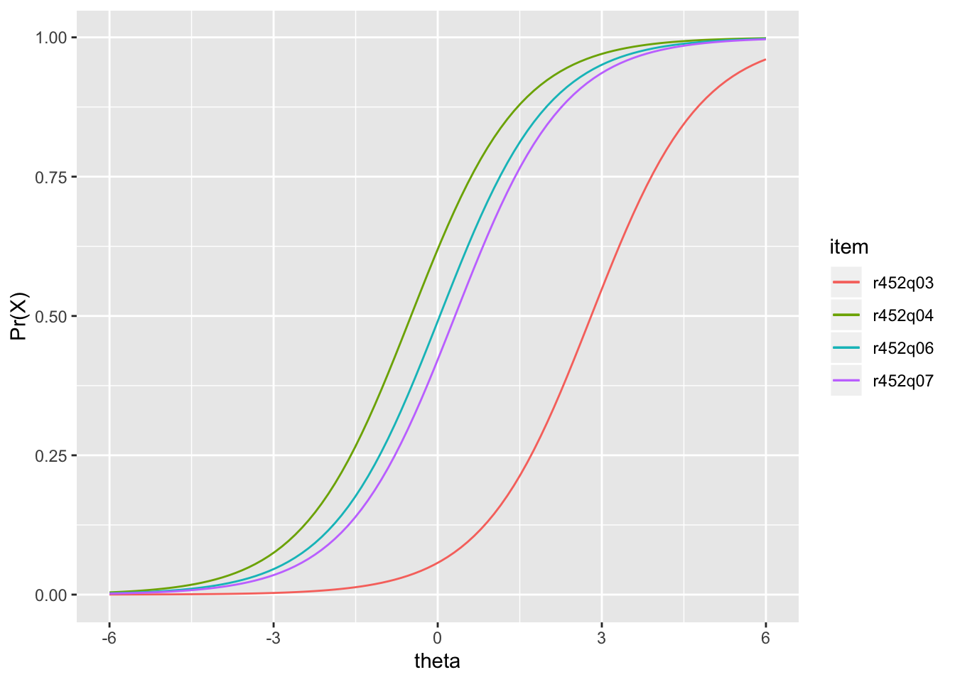
Figure 7.3: IRF for PISA09 reading items from “The play’s the thing” based on students in Great Britain.
Item pisagbr$r452q03s is estimated to be the most difficult for this set. The remaining three items in Figure 7.3 have locations or \(b\) parameters near theta 0. Notice that the IRF for these items, which come from the Rasch model, are all parallel, with the same slopes. They also have lower asymptotes of \(\Pr = 0\).
We can also use the results in irtgbr to examine SEM over theta. The SEM is obtained using the rtef() function from epmr. Figure 7.4 compares the SEM over theta for the full set of items (the black line), with SEM for subsets of 4 (blue) and 8 items (green). Fewer items at a given point in the theta scale also results in higher SEM at that theta. Thus, the number and location of items on the scale impact the resulting SEM.
# Plot SEM curve conditional on theta for full items
# Then add SEM for the subset of items 1:8 and 1:4
ggplot(rtef(irtgbr$ip), aes(theta, se)) + geom_line() +
  geom_line(aes(theta, se), data = rtef(irtgbr$ip[1:8, ]),
    col = "blue") +
  geom_line(aes(theta, se), data = rtef(irtgbr$ip[1:4, ]),
    col = "green")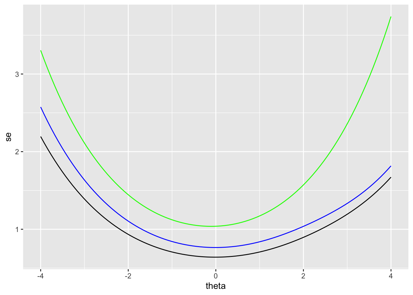
Figure 7.4: SEM for two subsets of PISA09 reading items based on students in Great Britain.
The rtef() function is used above with the default vector of theta seq(-4, 4, length = 100). However, SEM can be obtained for any theta based on the item parameters provided. Suppose we want to estimate the SEM for a high ability student who only takes low difficulty items. This constitutes a mismatch in item and construct, which produces a higher SEM. These SEM are interpreted like SEM from CTT, as the average variability we’d expect to see in a score due to measurement error. They can be used to build confidence intervals around theta for an individual.
# SEM for theta 3 based on the four easiest and the four
# most difficult items
rtef(irtgbr$ip[c(4, 6, 9, 11), ], theta = 3)
##   theta       se
## 1     3 2.900782
rtef(irtgbr$ip[c(2, 7, 8, 10), ], theta = 3)
##   theta       se
## 1     3 1.996224
The reciprocal of the SEM function, via the TEF, is the test information function. This simply shows us where on the theta scale our test items are accumulating the most discrimination power, and, as a result, where measurement will be the most accurate. Higher information corresponds to higher accuracy and lower SEM. Figure 7.5 shows the test information for all the reading items, again based on students in Great Britain. Information is highest where SEM is lowest, at the center of the theta scale.
# Plot the test information function over theta
# Information is highest at the center of the theta scale
ggplot(rtif(irtgbr$ip), aes(theta, i)) + geom_line()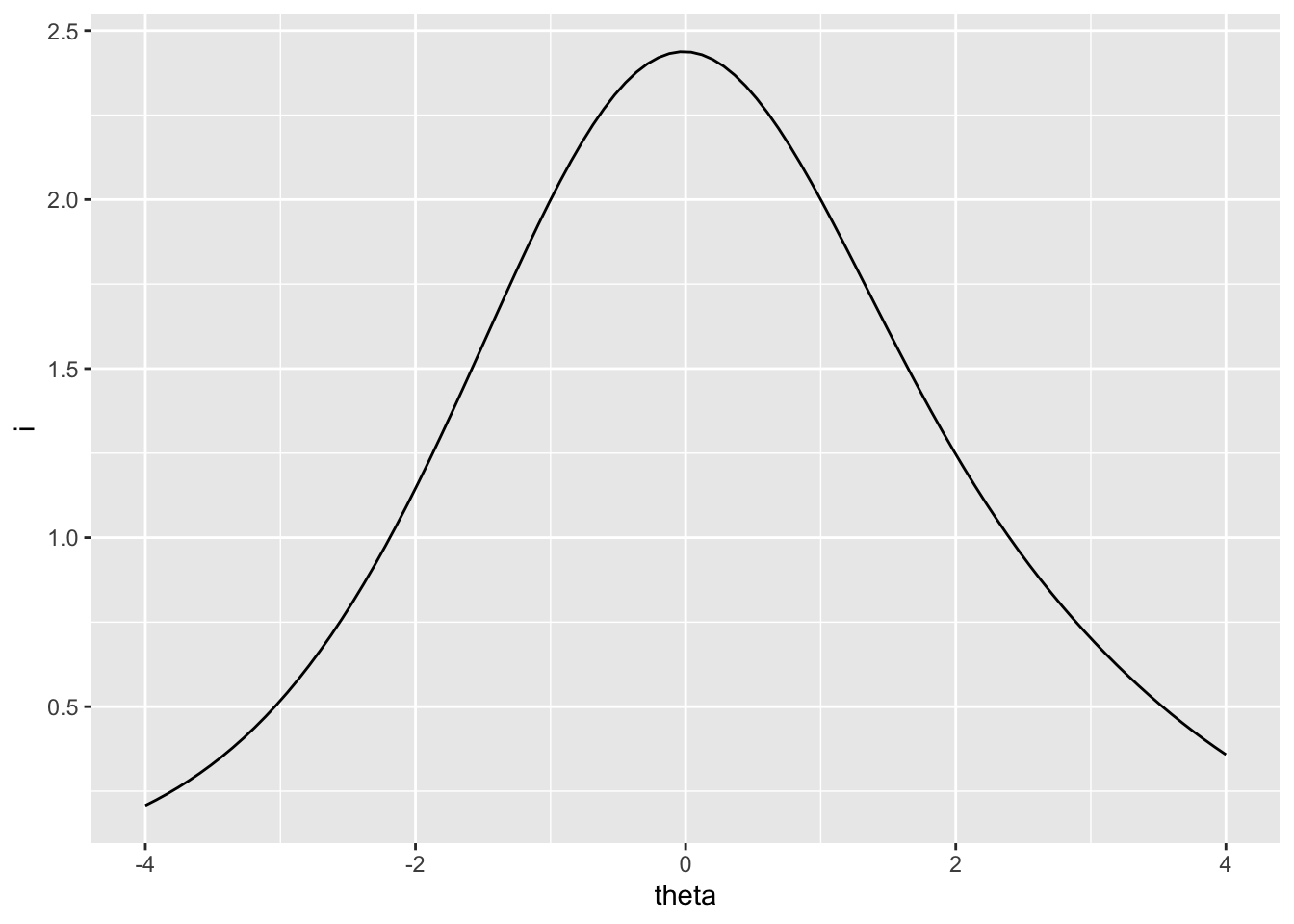
Figure 7.5: Test information for PISA09 reading items based on students in Great Britain.
Finally, just as the IRF can be used to predict probability of correct response on an item, given theta and the item parameters, the TRF can be used to predict total score given theta and parameters for each item in the test. The TRF lets us convert person theta back into the raw score metric for the test. Similar to the IRF, the TRF is asymptotic at 0 and the number of dichotomous items in the test, in this case, 11. Thus, no matter how high or how low theta, our predicted total score can’t exceed the bounds of the raw score scale. Figure 7.6 shows the test response function for the Great Britain results.
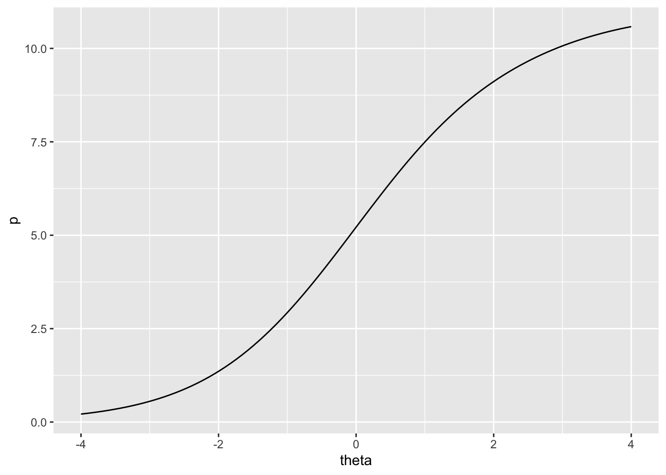
Figure 7.6: Test response function for PISA09 reading items based on students in Great Britain.
7.4 Summary
This chapter provided an introduction to IRT, with a comparison to CTT, and details regarding the three traditional, dichotomous, unidimensional IRT models. Assumptions of the models and some testing applications were presented. The Rasch model was demonstrated using data from PISA09, with examples of the IRF, TEF, TIF, and TRF.
7.4.1 Exercises
- Sketch out a plot of IRF for the following two items: a difficult item 1 with a high discrimination and negligible lower asymptote, and an easier item 2 with low discrimination and high lower asymptote. Be sure to label the axes of your plot.
- Sketch another plot of IRF for two items having the same difficulties, but different discriminations and lower asymptotes.
- Examine the IRF for the remaining
PISA09reading items for Great Britain. Check the content of the items in Appendix C to see what features of an item or prompt seemed to make it relatively easier or more difficult. - Using the
PISA09reading test results for Great Britain, find the predicted total scores associated with thetas of -1, 0, and 1. - Estimate the Rasch model for the
PISA09memorization strategies scale. First, dichotomize responses by recoding 1 to 0, and the remaining valid responses to 1. After fitting the model, plot the IRF for each item. - Based on the distribution of item difficulties for the memorization scale, where should SEM be lowest? Check the SEM by plotting the TEF for the full scale.
References
Bates, Douglas, Martin Mächler, Ben Bolker, and Steve Walker. 2015. “Fitting Linear Mixed-Effects Models Using lme4.” Journal of Statistical Software 67 (1): 1–48. https://doi.org/10.18637/jss.v067.i01.
de Ayala, R. J. 2009. The Theory and Practice of Item Response Theory. New York, NY: The Guilford Press.
De Boeck, Paul, Marjan Bakker, Robert Zwitser, Michel Nivard, Abe Hofman, Francis Tuerlinckx, and Ivailo Partchev. 2011. “The Estimation of Item Response Models with the Lmer Function from the Lme4 Package in R.” Journal of Statistical Software 39 (12): 1–28.
Doran, H., D. Bates, P. Bliese, and M. Dowling. 2007. “Estimating the Multilevel Rasch Model: With the Lme4 Package.” Journal of Statistical Software 20 (2): 1–18.
Embretson, S. E., and S. P. Reise. 2000. Item response theory for psychologists. Mahwah, NJ: Lawrence Erlbaum Associates.
Hambleton, R. K., and R. W. Jones. 1993. “Comparison of Classical Test Theory and Item Response Theory and Their Applications to Test Development.” Educational Measurement: Issues and Practice, 38–47.
Harvey, R. J., and A. L. Hammer. 1999. “Item Response Theory.” The Counseling Psychologist 27: 353–83.
Lord, F. M. 1952. “A theory of test scores.” Psychometric Monographs. No. 7.
Rasch, G. 1960. Probabilistic Models for Some Intelligence and Attainment Tests. Chicago, IL: University of Chicago Press.
Rizopoulos, Dimitris. 2006. “ltm: An R Package for Latent Variable Modelling and Item Response Theory Analyses.” Journal of Statistical Software 17 (5): 1–25. http://www.jstatsoft.org/v17/i05/.