Chapter 6 Item Analysis

Chapter 5 covered topics that rely on statistical analyses of data from educational and psychological measurements. These analyses are used to examine the relationships among scores on one or more test forms, in reliability, and scores based on ratings from two or more judges, in interrater reliability. Aside from coefficient alpha, all of the statistical analyses introduced so far focus on composite scores. Item analysis focuses instead on statistical analysis of the items themselves that make up these composites.

As discussed in Chapter 4, test items make up the most basic building blocks of an assessment instrument. Item analysis lets us investigate the quality of these individual building blocks, including in terms of how well they contribute to the whole and improve the validity of our measurement.

This chapter extends concepts from Chapters 2 and 5 to analysis of item performance within a CTT framework. The chapter begins with an overview of item analysis, including some general guidelines for preparing for an item analysis, entering data, and assigning score values to individual items. Some commonly used item statistics are then introduced and demonstrated. Finally, two additional item-level analyses are discussed, differential item functioning analysis and option analysis.

Learning objectives

Explain how item bias and measurement error negatively impact the quality of an item, and how item analysis, in general, can be used to address these issues.
Describe general guidelines for collecting pilot data for item analysis, including how following these guidelines can improve item analysis results.
Identify items that may have been keyed or scored incorrectly.
Recode variables to reverse their scoring or keyed direction.
Use the appropriate terms to describe the process of item analysis with cognitive vs noncognitive constructs.
Calculate and interpret item difficulties and compare items in terms of difficulty.
Calculate and interpret item discrimination indices, and describe what they represent and how they are used in item analysis.
Describe the relationship between item difficulty and item discrimination and identify the practical implications of this relationship.
Calculate and interpret alpha-if-item-deleted.
Utilize item analysis to distinguish between items that function well in a set and items that do not.
Remove items from an item set to achieve a target level of reliability.
Evaluate selected-response options using option analysis.

In this chapter, we’ll run item and option analyses on PISA09 data using epmr, with results plotted, as usual, using ggplot2.

# R setup for this chapter
# Required packages are assumed to be installed,
# see chapter 1
library("epmr")
library("ggplot2")
# Functions we'll use in this chapter
# str() for checking the structure of an object
# recode() for recoding variables
# colMeans() for getting means by column
# istudy() from epmr for running an item analysis
# ostudy() from epmr for running an option analysis
# subset() for subsetting data
# na.omit() for removing cases with missing data

6.1 Preparing for item analysis

6.1.1 Item quality

As noted above, item analysis lets us examine the quality of individual test items. Information about individual item quality can help us determine whether or not an item is measuring the content and construct that it was written to measure, and whether or not it is doing so at the appropriate ability level. Because we are discussing item analysis here in the context of CTT, we’ll assume that there is a single construct of interest, perhaps being assessed across multiple related content areas, and that individual items can contribute or detract from our measurement of that construct by limiting or introducing construct irrelevant variance in the form of bias and random measurement error.

Bias represents a systematic error with an influence on item performance that can be attributed to an interaction between examinees and some feature of the test. Bias in a test item leads examinees having a known background characteristic, aside from their ability, to perform better or worse on an item simply because of this background characteristic. For example, bias sometimes results from the use of scenarios or examples in an item that are more familiar to certain gender or ethnic groups. Differential familiarity with item content can make an item more relevant, engaging, and more easily understood, and can then lead to differential performance, even for examinees of the same ability level. We identify such item bias primarily by using measures of item difficulty and differential item functioning (DIF), discussed below and again in Chapter 7.

Bias in a test item indicates that the item is measuring some other construct besides the construct of interest, where systematic differences on the other construct are interpreted as meaningful differences on the construct of interest. The result is a negative impact on the validity of test scores and corresponding inferences and interpretations. Random measurement error on the other hand is not attributed to a specific identifiable source, such as a second construct. Instead, measurement error is inconsistency of measurement at the item level. An item that introduces measurement error detracts from the overall internal consistency of the measure, and this is detected in CTT, in part, using item analysis statistics.

6.1.2 Piloting

The goal in developing an instrument or scale is to identify bias and inconsistent measurement at the item level prior to administering a final version of our instrument. As we talk about item analysis, remember that the analysis itself is typically carried out in practice using pilot data. Pilot data are gathered prior to or while developing an instrument or scale. These data require at least a preliminary version of the educational or psychological measure. We’ve written some items for our measure, and we want to see how well they work.

Nunnally and Bernstein (1994) and others recommend that the initial pilot “pool” of candidate test items should be 1.5 to 2 times as large as the final number of items needed. So, if you’re envisioning a test with 100 items on it, you should aim to pilot 150 to 200 items. This may not be feasible, but it is a best-case scenario, and should at least be followed in large-scale testing. By collecting data on up to twice as many items as we intend to actually use, we’re acknowledging that, despite our best efforts, many of our preliminary test items may either be low quality, for example, biased or internally inconsistent, and they may address different ability levels or content than intended.

An adequate sample size of test takers is essential if we hope to obtain item analysis results that generalize to the population of test takers. Nunnally and Bernstein (1994) recommend that data be collected on at least 300 individuals from the population of interest, or 5 times as many individuals as test items, whichever is larger. A more practical goal for smaller scale testing applications, such as with classroom assessments, is 100 to 200 test takers. With smaller or non-representative samples, our item analysis results must be interpreted with caution. As with inferences made based on other types of statistics, small samples more often lead to erroneous results. Keep in mind that every statistic discussed here has a standard error and confidence interval associated with it, whether it is directly examined or not. Note also that bias and measurement error arise in addition to this standard error or sampling error, and we cannot identify bias in our test questions without representative data from our intended population. Thus, adequate sampling in the pilot study phase is critical.

The item analysis statistics discussed here are based on the CTT model of test performance. In Chapter 7 we’ll discuss the more complex item response theory (IRT) and its applications in item analysis.

6.1.3 Data entry

After piloting a set of items, raw item responses are organized into a data frame with test takers in rows and items in columns. The str() function is used here to summarize the structure of the unscored items on the PISA09 reading test. Each unscored item is coded in R as a factor with four to eight factor levels. Each factor level represents different information about a student’s response.

# Recreate the item name index and use it to check the 
# structure of the unscored reading items
# The strict.width argument is optional, making sure the
# results fit in the console window
ritems <- c("r414q02", "r414q11", "r414q06", "r414q09",
  "r452q03", "r452q04", "r452q06", "r452q07", "r458q01",
  "r458q07", "r458q04")
str(PISA09[, ritems], strict.width = "cut")
## 'data.frame':    44878 obs. of  11 variables:
##  $ r414q02: Factor w/ 7 levels "1","2","3","4",..: 2 1 4 1 1 2 2 2 3 2 ...
##  $ r414q11: Factor w/ 7 levels "1","2","3","4",..: 4 1 1 1 3 1 1 3 1 1 ...
##  $ r414q06: Factor w/ 5 levels "0","1","8","9",..: 1 4 2 1 2 2 2 4 1 1 ...
##  $ r414q09: Factor w/ 8 levels "1","2","3","4",..: 3 7 4 3 3 3 3 5 3 3 ...
##  $ r452q03: Factor w/ 5 levels "0","1","8","9",..: 1 4 1 1 1 2 2 1 1 1 ...
##  $ r452q04: Factor w/ 7 levels "1","2","3","4",..: 4 6 4 3 2 2 2 1 2 2 ...
##  $ r452q06: Factor w/ 4 levels "0","1","9","r": 1 3 2 1 2 2 2 2 1 2 ...
##  $ r452q07: Factor w/ 7 levels "1","2","3","4",..: 3 6 3 1 2 4 4 4 2 4 ...
##  $ r458q01: Factor w/ 7 levels "1","2","3","4",..: 4 4 4 3 4 4 3 4 3 3 ...
##  $ r458q07: Factor w/ 4 levels "0","1","9","r": 1 3 2 1 1 2 1 2 2 2 ...
##  $ r458q04: Factor w/ 7 levels "1","2","3","4",..: 2 3 2 3 2 2 2 3 3 4 ...

In addition to checking the structure of the data, it’s good practice to run frequency tables on each variable. An example is shown below for a subset of PISA09 reading items. The frequency distribution for each variable will reveal any data entry errors that resulted in incorrect codes. Frequency distributions should also match what we expect to see for correct and incorrect response patterns and missing data.

PISA09 items that include a code or factor level of “0” are constructed-response items, scored by raters. The remaining factor levels for these CR items are coded “1” for full credit, “7” for not administered, “9” for missing, and “r” for not reached, where the student ran out of time before responding to the item. Selected-response items do not include a factor level of “0.” Instead, they contain levels “1” through up to “5,” which correspond to multiple-choice options one through five, and then codes of “7” for not administered, “8” for an ambiguous selected response, “9” for missing, and “r” again for not reached.

# Subsets of the reading item index for constructed and
# selected items
# Check frequency tables by item (hence the 2 in apply)
# for CR items
critems <- ritems[c(3, 5, 7, 10)]
sritems <- ritems[c(1:2, 4, 6, 8:9, 11)]
apply(PISA09[, critems], 2, table, exclude = NULL)
##   r414q06 r452q03 r452q06 r458q07
## 0    9620   33834   10584   12200
## 1   23934    5670   22422   25403
## 9   10179    4799   11058    6939
## r    1145     575     814     336

In the piloting and data collection processes, response codes or factor levels should be chosen carefully to represent all of the required response information. Responses should always be entered in a data set in their most raw form. Scoring should then happen after data entry, through the creation of new variables, whenever possible.

6.1.4 Scoring

In Chapter 2, which covered measurement, scales, and scoring, we briefly discussed the difference between dichotomous and polytomous scoring. Each involves the assignment of some value to each possible observed response to an item. This value is taken to indicate a difference in the construct underlying our measure. For dichotomous items, we usually assign a score of 1 to a correct response, and a zero otherwise. Polytomous items involve responses that are correct to differing degrees, for example, 0, 1, and 2 for incorrect, somewhat correct, and completely correct.

In noncognitive testing, we replace “correctness” from the cognitive context with “amount” of the trait or attribute of interest. So, a dichotomous item might involve a yes/no response, where “yes” is taken to mean the construct is present in the individual, and it is given a score of 1, whereas “no” is taken to mean the construct is not present, and it is given a score of 0. Polytomous items then allow for different amounts of the construct to be present.

Although it seems standard to use dichotomous 0/1 scoring, and polytomous scoring of 0, 1, 2, ect., these values should not be taken for granted. The score assigned to a particular response determines how much a given item will contribute to any composite score that is later calculated across items. In educational testing, the typical scoring schemes are popular because they are simple. Other scoring schemes could also be used to given certain items more or less weight when calculating the total.

For example, a polytomous item could be scored using partial credit, where incorrect is scored as 0, completely correct is given 1, and levels of correctness are assigned decimal values in between. In psychological testing, the center of the rating scale could be given a score of 0, and the tails could decrease and increase from there. For example, if a rating scale is used to measure levels of agreement, 0 could be assigned to a “neutral” rating, and -2 and -1 might correspond to “strongly disagree” and “disagree,” with 1 and 2 corresponding to “agree” and “strongly agree.” Changing the values assigned to item responses in this way can help improve the interpretation of summary results.

Scoring item responses also requires that direction, that is, decreases and increases, be given to the correctness or amount of trait involved. Thus, at the item level, we are at least using an ordinal scale. In cognitive testing, the direction is simple: increases in points correspond to increases in correctness. In psychological testing, reverse scoring may also be necessary.

PISA09 contains examples of scoring for both educational and psychological measures. First, we’ll check the scoring for the CR and SR reading items. A crosstab for the raw and scored versions of an item shows how each code was converted to a score. Note students not reaching an item, with an unscored factor level “r”, were given an NA for their score.

# Indices for scored reading items
rsitems <- paste0(ritems, "s")
crsitems <- paste0(critems, "s")
srsitems <- paste0(sritems, "s")
# Tabulate unscored and scored responses for the first CR
# item
# exclude = NULL shows us NAs as well
# raw and scored are not arguments to table, but are used
# simply to give labels to the printed output
table(raw = PISA09[, critems[1]],
  scored = PISA09[, crsitems[1]],
  exclude = NULL)
##    scored
## raw     0     1  <NA>
##   0  9620     0     0
##   1     0 23934     0
##   8     0     0     0
##   9 10179     0     0
##   r     0     0  1145
# Create the same type of table for the first SR item

For a psychological example, we revisit the attitude toward school items presented in Figure 2.2. In PISA09, these items were coded during data entry with values of 1 through 4 for “Strongly Disagree” to “Strongly Agree.” We could utilize these as the scored responses in the item analyses that follow. However, we first need to recode the two items that were worded in the opposite direction as the others. Then, higher scores on all four items will represent more positive attitudes toward school.

# Check the structure of raw attitude items
str(PISA09[, c("st33q01", "st33q02", "st33q03",
  "st33q04")])
## 'data.frame':    44878 obs. of  4 variables:
##  $ st33q01: num  3 3 2 1 2 2 2 3 2 3 ...
##  $ st33q02: num  2 2 1 1 2 2 2 2 1 2 ...
##  $ st33q03: num  2 1 3 3 3 3 1 3 1 3 ...
##  $ st33q04: num  3 3 4 3 3 3 3 2 1 3 ...
# Rescore two items
PISA09$st33q01r <- recode(PISA09$st33q01)
PISA09$st33q02r <- recode(PISA09$st33q02)

6.2 Traditional item statistics

Three statistics are commonly used to evaluate the items within a scale or test. These are item difficulty, discrimination, and alpha-if-item-deleted. Each is presented below with examples based on PISA09.

6.2.1 Item difficulty

Once we have established scoring schemes for each item in our test, and we have applied them to item-response data from a sample of individuals, we can utilize some basic descriptive statistics to examine item-level performance. The first statistic is item difficulty, or, how easy or difficult each item is for our sample. In cognitive testing, we talk about easiness and difficulty, where test takers can get an item correct to different degrees, depending on their ability or achievement. In noncognitive testing, we talk instead about endorsement or likelihood of choosing the keyed response on the item, where test takers are more or less likely to endorse an item, depending on their level on the trait. In the discussions that follow, ability and trait can be used interchangeably, as can correct/incorrect and keyed/unkeyed response, and difficulty and endorsement. See Table 6.1 for a summary of these terms.

Table 6.1: Comparing Terms in Cognitive vs Noncognitive Item Analysis
General Term	Cognitive	Noncognitive
Construct	Ability	Trait
Levels on construct	Correct and incorrect	Keyed and unkeyed
Item performance	Difficulty	Endorsement

In CTT, the item difficulty is simply the mean score for an item. For dichotomous 0/1 items, this mean is referred to as a $p$-value, since it represents the proportion of examinees getting the item correct or choosing the keyed response. With polytomous items, the mean is simply the average score. When testing noncognitive traits, the term $p$-value may still be used. However, instead of item difficulty we refer to endorsement of the item, with proportion correct instead becoming proportion endorsed.

Looking ahead to IRT, item difficulty will be estimated as the predicted mean ability required to have a 50% chance of getting the item correct or endorsing the item.

Here, we calculate $p$-values for the scored reading items, by item type. Item PISA09$r452q03, a CR item, stands out from the rest as having a very low $p$-value of 0.13. This tells us that only 13% of students who took this item got it right. The next lowest $p$-value was 0.37.

# Get p-values for reading items by type
round(colMeans(PISA09[, crsitems], na.rm = T), 2)
## r414q06s r452q03s r452q06s r458q07s 
##     0.55     0.13     0.51     0.57
round(colMeans(PISA09[, srsitems], na.rm = T), 2)
## r414q02s r414q11s r414q09s r452q04s r452q07s r458q01s r458q04s 
##     0.49     0.37     0.65     0.65     0.48     0.56     0.59

For item r452q03, students read a short description of a scene from The Play’s the Thing, shown in Appendix C. The question then is, “What were the characters in the play doing just before the curtain went up?” This question is difficult, in part, because the word “curtain” is not used in the scene. So, the test taker must infer that the phrase “curtain went up” refers to the start of a play. The question is also difficult because the actors in this play are themselves pretending to be in a play. For additional details on the item and the rubric used in scoring, see Appendix C.

Although difficult questions may be frustrating for students, sometimes they’re necessary. Difficult or easy items, or items that are difficult or easy to endorse, may be required given the purpose of the test. Recall that the purpose of a test describes: the construct, what we’re measuring; the population, with whom the construct is being measured; and the application or intended use of scores. Some test purposes can only be met by including some very difficult or very easy items. PISA, for example, is intended to measure students along a continuum of reading ability. Without difficult questions, more able students would not be measured as accurately. On the other hand, a test may be intended to measure lower level reading skills, which many students have already mastered. In this case, items with high $p$-values would be expected. Without them, low ability students, who are integral to the test purpose, would not be able to answer any items correctly.

This same argument applies to noncognitive testing. To measure the full range of a clinical disorder, personality trait, or attitude, we need items that can be endorsed by individuals all along the continuum for our construct. Consider again the attitude toward school scale. All four items have mean scores above 2. On average, students agree with these attitude items, after reverse coding the first two, more often than not. If we recode scores to be dichotomous, with disagreement as 0 and agreement as 1, we can get $p$-values for each item as well. These $p$-values are interpreted as agreement rates. They tell us that at least 70% of students agreed with each attitude statement.

# Index for attitude toward school items, with the first
# two items recoded
atsitems <- c("st33q01r", "st33q02r", "st33q03",
  "st33q04")
# Check mean scores
round(colMeans(PISA09[, atsitems], na.rm = T), 2)
## st33q01r st33q02r  st33q03  st33q04 
##     3.04     3.38     2.88     3.26
# Convert polytomous to dichotomous, with any disagreement
# coded as 0 and any agreement coded as 1
ats <- apply(PISA09[, atsitems], 2, recode,
  list("0" = 1:2, "1" = 3:4))
round(colMeans(ats, na.rm = T), 2)
## st33q01r st33q02r  st33q03  st33q04 
##     0.78     0.92     0.77     0.89

Given their high means and $p$-values, we might conclude that these items are not adequately measuring students with negative attitudes toward school, assuming such students exist. Perhaps if an item were worded differently or were written to ask about another aspect of schooling, such as the value of homework, more negative attitudes would emerge. On the other hand, it could be that students participating in PISA really do have overall positive attitudes toward school, and regardless of the question they will tend to have high scores.

This brings us to one of the major limitations of CTT item analysis: the item statistics we compute are dependent on our sample of test takers. For example, we assume a low $p$-value indicates the item was difficult, but it may have simply been difficult for individuals in our sample. What if our sample happens to be lower on the construct than the broader population? Then, the items would tend to have lower means and $p$-values. If administered to a sample higher on the construct, item means would be expected to increase. Thus, the difficulty of an item is dependent on the ability of the individuals taking it.

Because we estimate item difficulty and other item analysis statistics without accounting for the ability or trait levels of individuals in our sample, we can never be sure of how sample-dependent our results really are. This sample dependence in CTT will be addressed in IRT.

6.2.2 Item discrimination

Whereas item difficulty tell us the mean level of performance on an item, across everyone taking the item, item discrimination tells us how item difficulty changes for individuals of different abilities. Discrimination extends item difficulty by describing mean item performance in relation to individuals’ levels of the construct. Highly discriminating cognitive items are easier for high ability students, but more difficult for low ability students. Highly discriminating noncognitive items are endorsed less frequently by test takers low on the trait, but more frequently by test takers high on the trait. In either case, a discriminating item is able to identify levels on the construct of interest, because scores on the item itself are positively related to the construct.

Item discrimination is measured by comparing performance on an item for different groups of people, where groups are defined based on some measure of the construct. In the early days of item analysis, these groups were simply defined as “high” and “low” using a cutoff on the construct to distinguish the two. If we knew the true abilities for a group of test takers, and we split them into two ability groups, we could calculate and compare $p$-values for a given item for each group. If an item were highly discriminating, we would expect it to have a higher $p$-value in the high ability group than in the low ability group. We would expect the discrepancy in $p$-values to be large. On the other hand, for an item that doesn’t discriminate well, the discrepancy between $p$-values would be small.

# Get total reading scores and check descriptives
PISA09$rtotal <- rowSums(PISA09[, rsitems])
dstudy(PISA09$rtotal)
## 
## Descriptive Study
## 
##   mean median   sd   skew kurt min max     n na
## x 5.57      6 2.86 -0.106    2   0  11 43628  0
# Compare CR item p-values for students below vs above the
# median total score
round(colMeans(PISA09[PISA09$rtotal <= 6, crsitems],
  na.rm = T), 2)
## r414q06s r452q03s r452q06s r458q07s 
##     0.32     0.03     0.28     0.39
round(colMeans(PISA09[PISA09$rtotal > 6, crsitems],
  na.rm = T), 2)
## r414q06s r452q03s r452q06s r458q07s 
##     0.87     0.27     0.84     0.83

Although calculating $p$-values for different groups of individuals is still a useful approach to examining item discrimination, we lose information when we reduce scores on our construct to categories such as “high” and “low.” Item discrimination is more often estimated using the correlation between item responses and construct scores. In the absence of scores on the construct, total scores are typically used as a proxy. The resulting correlation is referred to as an item-total correlation (ITC). When responses on the item are dichotomously scored, it is also sometimes called a point-biserial correlation.

Here, we take a subset of PISA09 including CR item scores and the total reading score for German students. We then omit all students with missing data using na.omit(). The correlation matrix for these five variables shows how scores on the items relate to one another, and to the total score. Relationships between items and the total are ITC estimates of item discrimination. The first item, with ITC of 0.7, is best able to discriminate between students of high and low ability.

# Create subset of data for German students, then reduce
# to complete data
pisadeu <- subset(PISA09, subset = cnt == "DEU",
  select = c(crsitems, "rtotal"))
pisadeu <- na.omit(pisadeu)
round(cor(pisadeu), 2)
##          r414q06s r452q03s r452q06s r458q07s rtotal
## r414q06s     1.00     0.27     0.42     0.39   0.70
## r452q03s     0.27     1.00     0.31     0.19   0.49
## r452q06s     0.42     0.31     1.00     0.31   0.65
## r458q07s     0.39     0.19     0.31     1.00   0.56
## rtotal       0.70     0.49     0.65     0.56   1.00

Note that when you correlate something with itself, the result should be a correlation of 1. When you correlate a component score, like an item, with a composite that includes that component, the correlation will increase simply because of the component in on both sides of the relationship. Correlations between item responses and total scores can be “corrected” for this spurious increase simply by excluding a given item when calculating the total. The result is referred to as a corrected item-total correlation (CITC). ITC and CITC are typically positively related with one another, and give relatively similar results. However, CITC is preferred, as it is considered more a conservative and more accurate estimate of discrimination.

Figure 6.1 contains scatter plots for two CR reading items from PISA09, items r414q06s and r452q03s. On the x-axis in each plot are total scores across all reading items, and on the y-axis are the scored item responses for each item. These plots help us visualize both item difficulty and discrimination. Difficulty is the amount of data horizontally aligned with 0, compared to 1, on the y-axis. More data points at 0 indicate more students getting the item wrong. Discrimination is then the bunching of data points at the low end of the x-axis for 0, and at the high end for 1.

# Scatter plots for visualizing item discrimination
ggplot(pisadeu, aes(rtotal, factor(r414q06s))) +
  geom_point(position = position_jitter(w = 0.2, h = 0.2))
ggplot(pisadeu, aes(rtotal, factor(r452q03s))) +
  geom_point(position = position_jitter(w = 0.2, h = 0.2))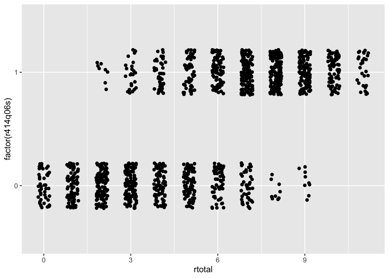

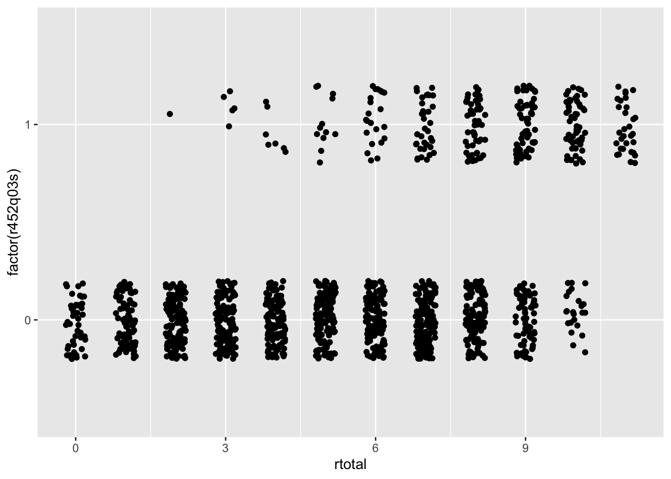
Scatter plots showing the relationship between total scores on the x-axis with dichotomous item response on two PISA items on the y-axis.

Figure 6.1: Scatter plots showing the relationship between total scores on the x-axis with dichotomous item response on two PISA items on the y-axis.

Suppose you had to guess a student’s reading ability based only on their score from a single item. Which of the two items shown in Figure 6.1 would best support your guess? Here’s a hint: it’s not item r452q03. Notice how students who got item r452q03 wrong have rtotal scores that span almost the entire score scale? People with nearly perfect scores still got this item wrong. On the other hand, item r414q06 shows a faster tapering off of students getting the item wrong as total scores increase, with a larger bunching of students of high ability scoring correct on the item. So, item r414q06, has a higher discrimination, and gives us more information about the construct than item r452q03.

Next, we calculate the ITC and CITC “by hand” for the first attitude toward school item, which was reverse coded as st33q01r. There is a sizable difference between the ITC and the CITC for this item, likely because the scale is so short to begin with. By removing the item from the total score, we reduce our scale length by 25%, and, presumably, our total score becomes that much less representative of the construct. Discrimination for the remaining attitude items will be examined later.

# Caculate ITC and CITC by hand for one of the attitude
# toward school items
PISA09$atstotal <- rowSums(PISA09[, atsitems])
cor(PISA09$atstotal, PISA09$st33q01r, use = "c")
## [1] 0.7325649
cor(PISA09$atstotal - PISA09$st33q01r,
  PISA09$st33q01r, use = "c")
## [1] 0.4659522

Although there are no clear guidelines on acceptable or ideal levels of discrimination, 0.30 is sometimes used as a minimum. This minimum can decrease to 0.20 or 0.15 in lower-stakes settings where other constructs like motivation are expected to impact the quality of our data. Typically, the higher the discrimination, the better. However, when correlations between item scores and construct scores exceed 0.90 and approach 1.00, we should question how distinct our item really is from the construct. Items that correlate too strongly with the construct could be considered redundant and unnecessary.

6.2.3 Internal consistency

The last item analysis statistic we’ll consider here indexes how individual items impact the overall internal consistency reliability of the scale. Internal consistency is estimated via coefficient alpha, introduced in Chapter 5. Alpha tells us how well our items work together as a set. “Working together” refers to how consistently the item responses change, overall, in similar ways. A high coefficient alpha tells us that people tend to respond in similar ways from one item to the next. If coefficient alpha were perfectly 1.00, we would know that each person responded in exactly the same rank-ordered way across all items. An item’s contribution to internal consistency is measured by estimating alpha with that item removed from the set. The result is a statistic called alpha-if-item-deleted (AID).

AID answers the question, what happens to the internal consistency of a set of items when a given item is removed from the set? Because it involves the removal of an item, higher AID indicates a potential increase in internal consistency when an item is removed. Thus, when it is retained, the item is actually detracting from the internal consistency of the scale. Items that detract from the internal consistency should be considered for removal.

To clarify, it is bad news for an item if the AID is higher than the overall alpha for the full scale. It is good news for an item if AID is lower than alpha for the scale.

The istudy() function in the epmr package estimates AID, along with the other item statistics presented so far. AID is shown in the last column of the output. For the PISA09 reading items, the overall alpha is 0.7597, which is an acceptable level of internal consistency for a low-stakes measure like this (see Table 5.1). The AID results then tell us that alpha never increases beyond its original level after removing individual items, so, good news. Instead, alpha decreases to different degrees when items are removed. The lowest AID is 0.7252 for item r414q06. Removal of this item results in the largest decrease in internal consistency.

# Estimate item analysis statistics, including alpha if
# item deleted
istudy(PISA09[, rsitems])
## 
## Scored Item Study
## 
## Alpha: 0.7597 
## 
## Item statistics:
##              m    sd     n   na   itc  citc   aid
## r414q02s 0.494 0.500 43958  920 0.551 0.411 0.742
## r414q11s 0.375 0.484 43821 1057 0.455 0.306 0.755
## r414q06s 0.547 0.498 43733 1145 0.652 0.533 0.725
## r414q09s 0.653 0.476 43628 1250 0.518 0.380 0.745
## r452q03s 0.128 0.334 44303  575 0.406 0.303 0.753
## r452q04s 0.647 0.478 44098  780 0.547 0.413 0.741
## r452q06s 0.509 0.500 44064  814 0.637 0.515 0.728
## r452q07s 0.482 0.500 43979  899 0.590 0.458 0.735
## r458q01s 0.556 0.497 44609  269 0.505 0.360 0.748
## r458q07s 0.570 0.495 44542  336 0.553 0.416 0.741
## r458q04s 0.590 0.492 44512  366 0.522 0.381 0.745

Note that discrimination and AID are typically positively related with one another. Discriminating items tend also to contribute to internal consistency. However, these two item statistics technically measure different things, and they need not correspond to one another. Thus, both should be considered when evaluating items in practice.

6.2.4 Item analysis applications

Now that we’ve covered the three major item analysis statistics, difficulty, discrimination, and contribution to internal consistency, we need to examine how they’re used together to build a set of items. All of the scales in PISA09 have already gone through extensive piloting and item analysis, so we’ll work with a hypothetical scenario to make things more interesting.

Suppose we needed to identify a brief but effective subset of PISA09 reading items for students in Hong Kong. The items will be used in a low-stakes setting where practical constraints limit us to only eight items, so long as those eight items maintain an internal consistency reliability at or above 0.60. First, let’s use the Spearman-Brown formula to predict how low reliability would be expected to drop if we reduced our test length from eleven to eight items.

# Subset of data for Hong Kong, scored reading items
pisahkg <- subset(PISA09, cnt == "HKG", rsitems)
# Spearman-Brown based on original alpha and new test
# length of 8 items
sb_r(r = coef_alpha(pisahkg)$alpha, k = 8/11)
## [1] 0.6049326

Our new reliability is estimated to be 0.605, which, thankfully, meets our hypothetical requirements. Now, we can explore our item statistics to find items for removal. The item analysis results for the full set of eleven items show two items with CITC below 0.20. These are items r414q11 and r452q03. These items also have AID near or above alpha for the full set, indicating that both are detracting from the internal consistency of the measure, though only to a small degree. Finally, notice that these are also the most difficult items in the set, with means of 0.36 and 0.04 respectively. Only 4% of students in Hong Kong got item r452q03 right.

# Item analysis for Hong Kong
istudy(pisahkg)
## 
## Scored Item Study
## 
## Alpha: 0.678 
## 
## Item statistics:
##               m    sd    n na   itc  citc   aid
## r414q02s 0.5109 0.500 1474 10 0.496 0.322 0.658
## r414q11s 0.3553 0.479 1469 15 0.349 0.165 0.685
## r414q06s 0.6667 0.472 1467 17 0.596 0.452 0.634
## r414q09s 0.7019 0.458 1466 18 0.439 0.273 0.666
## r452q03s 0.0405 0.197 1481  3 0.233 0.156 0.679
## r452q04s 0.6295 0.483 1479  5 0.541 0.382 0.646
## r452q06s 0.6303 0.483 1477  7 0.586 0.435 0.637
## r452q07s 0.4830 0.500 1474 10 0.510 0.338 0.654
## r458q01s 0.5037 0.500 1481  3 0.481 0.305 0.660
## r458q07s 0.5922 0.492 1481  3 0.515 0.349 0.652
## r458q04s 0.6914 0.462 1481  3 0.538 0.386 0.646

Let’s remove these two lower-quality items and check the new results. The means and SD should stay the same for this new item analysis. However, the remaining statistics, ITC, CITC, and AID, all depend on the full set, so we would expect them to change. The results indicate that all of our AID are below alpha for the full set of nine items. The CITC are acceptable for a low-stakes test. However, item item r414q09 has the weakest discrimination, making it the best candidate for removal, all else equal.

# Item analysis for a subset of items 
istudy(pisahkg[, rsitems[-c(2, 5)]])
## 
## Scored Item Study
## 
## Alpha: 0.6874 
## 
## Item statistics:
##              m    sd    n na   itc  citc   aid
## r414q02s 0.511 0.500 1474 10 0.506 0.320 0.670
## r414q06s 0.667 0.472 1467 17 0.605 0.451 0.643
## r414q09s 0.702 0.458 1466 18 0.454 0.277 0.678
## r452q04s 0.629 0.483 1479  5 0.542 0.370 0.659
## r452q06s 0.630 0.483 1477  7 0.601 0.442 0.645
## r452q07s 0.483 0.500 1474 10 0.514 0.330 0.668
## r458q01s 0.504 0.500 1481  3 0.500 0.314 0.671
## r458q07s 0.592 0.492 1481  3 0.537 0.361 0.661
## r458q04s 0.691 0.462 1481  3 0.550 0.388 0.656

Note that the reading items included in PISA09 were not developed to function as a reading scale. Instead, these are merely a sample of items from the study, the items with content that was made publicly available. Also, in practice, an item analysis will typically involve other considerations besides the statistics we are covering here, most importantly, content coverage. Before removing an item from a set, we should consider how the test outline will be impacted, and whether or not the balance of content is still appropriate.

6.3 Additional analyses

Whereas item analysis is useful for evaluating the quality of items and their contribution to a test or scale, other analyses are available for digging deeper into the strengths and weaknesses of items. Two commonly used analyses are option analysis, also called distractor analysis, and differential item functioning analysis.

6.3.1 Option analysis

So far, our item analyses have focused on scored item responses. However, data from unscored SR items can also provide useful information about test takers. An option analysis involves the examination of unscored item responses by ability or trait groupings for each option in a selected-response item. Relationships between the construct and response patters over keyed and unkeyed options can give us insights into whether or not response options are functioning as intended.

To conduct an option analysis, we simply calculate bivariate (two variables) frequency distributions for ability or trait levels (one variable) and response choice (the other variable). Response choice is already a nominal variable, and the ability or trait is usually converted to ordinal categories to simplify interpretation.

The ostudy() function from epmr takes a matrix of unscored item responses, along with some information about the construct (a grouping variable, a vector of ability or trait scores, or a vector containing the keys for each item) and returns crosstabs for each item that break down response choices by construct groupings. By default, the construct is categorized into three equal-interval groups, with labels “low”, “mid”, and “high.”

# Item option study on all SR reading items
pisao <- ostudy(PISA09[, sritems], scores = PISA09$rtotal)
# Print frequency results for one item
pisao$counts$r458q04
##    groups
##       low   mid  high
##   1  2117   890   297
##   2  5039  9191 11608
##   3  5288  2806   855
##   4  2944  1226   266
##   8   224    73    18
##   9   658   110    18
##   r     0     0     0

With large samples, a crosstab of counts can be difficult to interpret. Instead, we can also view percentages by option, in rows, or by construct group, in columns. Here, we check the percentages by column, where each column should sum to 100%. These results tell us the percentage of students within each ability group that chose each option.

# Print option analysis percentages by column
# This item discriminates relatively well
pisao$colpct$r458q04
##    groups
##     low mid high
##   1  13   6    2
##   2  31  64   89
##   3  33  20    7
##   4  18   9    2
##   8   1   1    0
##   9   4   1    0
##   r   0   0    0

Consider the distribution over response choices for high ability students, in the last column of the crosstab for item r458q04. The large majority of high ability students, 89%, chose the second option on this item, which is also the correct or keyed option. On the other hand, low ability students, in the left column of the crosstab, are spread out across the different options, with only 31% choosing the correct option. This is what we hope to see for an item that discriminates well.

# Print option analysis percentages by column
# This item discriminates relatively less well
pisao$colpct$r414q11
##    groups
##     low mid high
##   1  44  51   29
##   2  25   8    2
##   3  16  35   67
##   4   9   5    2
##   8   1   0    0
##   9   5   1    0
##   r   0   0    0

Item r414q11 doesn’t discriminate as well as item r458q04, and this is reflected in the option analysis results. The majority of high ability students are still choosing the correct option. However, some are also pulled toward another, incorrect option, option 1. The majority of low ability students are choosing option 1, with fewer choosing the correct option.

In addition to telling us more about the discrimination of an item by option, these results also help us identify dysfunctional options, ones which do not provide us with any useful information about test takers. Do you see any options in item r414q11 that don’t function well? The incorrect options are 1, 2, and 4.

A dysfunctional option is one that fails to attract the students we expect to choose it. We expect high ability students to choose the correct option. On more difficult questions, we also expect some high ability students to choose one or more incorrect options. We typically expect a somewhat uniform distribution of choices for low ability students. If our incorrect options were written to capture common misunderstandings of students, we may expect them to be chosen by low ability students more often than the correct option. A dysfunctional incorrect option is then one that is chosen by few low or medium ability students, or is chosen by high ability students more often than the correct option.

When an incorrect option is infrequently or never chosen by lower ability groups, it is often because the option is obviously incorrect. In item r414q11, option 4 is chosen by only 9% of low ability students and 5% of medium ability students. Reviewing the content of the item in Appendix C.1, the option (D) doesn’t stand out as being problematic. It may have been better worded as “It proves the No argument.” Then, it would have conformed with the wording in option 2 (B). However, the option appears to follow the remaining item writing guidelines.

6.3.2 Differential item functioning

A second supplemental item analysis, frequently conducted with large-scale and commercially available tests, is an analysis of differential item functioning or DIF. Consider a test question where students of the same ability or trait level respond differently based on certain demographic or background features pertaining to the examinee, but not relating directly to the construct. In an option analysis, we examine categorical frequency distributions for each response option by ability groups. In DIF, we examine these same categorical frequency distributions, but by different demographic groups, where all test takers in the analysis have the same level on the construct. The presence of DIF in a test item is evidence of potential bias, as, after controlling for the construct, demographic variables should not produce significant differences in test taker responses.

A variety of statistics, with R packages to calculate them, are available for DIF analysis in educational and psychological testing. We will not review them all here. Instead, we focus on the concept of DIF and how it is displayed in item level performance in general. We’ll return to this discussion in Chapter 7, within IRT.

DIF is most often based on a statistical model that compares item difficulty or the mean performance on an item for two groups of test takers, after controlling for their ability levels. Here, controlling for refers to either statistical or experimental control. The point is that we in some way remove the effects of ability on mean performance per group, so that we can then examine any leftover performance differences. Testing for the significance of DIF can be done, for example, using IRT, logistic regression, or chi-square statistics. Once DIF is identified for an item, the item itself is examined for potential sources of differential performance by subgroup. The item is either rewritten or deleted.

6.4 Summary

This chapter provided an introduction to item analysis in cognitive and noncognitive testing, with some guidelines on collecting and scoring pilot data, and an overview of five types of statistics used to examine item level performance, including item difficulty, item discrimination, internal consistency, option analysis, and differential item functioning. These statistics are used together to identify items that contribute or detract from the quality of a measure.

Item analysis, as described in this chapter, is based on a CTT model of test performance. We have assumed that a single construct is being measured, and that item analysis results are based on a representative sample from our population of test takers. Chapter 7 builds on the concepts introduced here by extending them to the more complex but also more popular IRT model of test performance.

6.4.1 Exercises

Explain why we should be cautious about interpreting item analysis results based on pilot data.
For an item with high discrimination, how should $p$-values on the item compare when calculated separately for two groups that differ in their true mean abilities?
Why is discrimination usually lower for CITC as compared with ITC for a given item?
What features of certain response options, in terms of the item content itself, would make them stand out as problematic within a option analysis?
Explain how AID is used to identify items contributing to internal consistency.
Conduct an item analysis on the PISA09 reading items for students in Great Britain (PISA09$cnt == "GBR"). Examine and interpret results for item difficulty, discrimination, and AID.
Conduct a option analysis on SR reading item r414q09, with an interpretation of results.

References

Nunnally, J. C, and I. H. Bernstein. 1994. Psychometric Theory. New York, NY: McGraw-Hill.